Exercise 5: Processing Data (CDC)

Author

Asmith Joseph

Published

February 2, 2025

Data Source Description

The National Artesunate for Severe Malaria Program Case Report Data (April - December 2019) provides deidentified patient data on individuals receiving intravenous (IV) artesunate, the first-line treatment for severe malaria. Collected through the Centers for Disease Control and Prevention (CDC), this dataset contains 197 observations and 119 clinical variables, detailing malaria diagnosis methods, organ dysfunction indicators, laboratory values, and treatment responses. Each patient is assigned a unique ParticipantID, which allows linkage to related datasets, including Artesun ate Dosing Data, Follow-On Antimalarial Dosing Data, and Microscopy (Parasitemia) Data. The dataset, last updated on April 10, 2020, is publicly available on the CDC open data portal (https://data.cdc.gov/Global-Health/National-Artesunate-for-Severe-Malaria-Program-Cas/igaz-icki/about_data). Key variables include Dx (diagnosis method), IV_parasitemia (malaria confirmation), IV_shock (shock status), IV_ards (Acute Respiratory Distress Syndrome), IV_ARF (Acute Renal Failure), and IV_DIC (Disseminated Intravascular Coagulation). Additionally, it includes a Data Dictionary and a Guide to NASMP Datasets, offering comprehensive documentation for analysis.

Explanations of Downloading and saving the dataset. See below for the code!

To work with this dataset, the first step is I download the dataset from the CDC Open Data Portal in CSV format. This is done by defining the dataset’s URL and using R’s read_csv() function to import it into a dataframe. Once the data is loaded, the head() function is used to preview the first few rows, and the View() function allows for manual inspection in RStudio’s data viewer. After confirming that the dataset has been successfully retrieved, the next step is to save it locally for easier access. To do this, a local file path is specified, ensuring that the dataset is stored in a designated folder on the computer. The write_csv() function is then used to save the dataframe as a CSV file in the specified directory.

Downloading the data.

#Installing necessary libraries to read the OData Atom XML feed (It is a is a structured XML document used for exposing and consuming data via OData APIs)
# Installing necessary libraries to read the OData Atom XML feed

# Load libraries
library(httr)

Warning: package 'httr' was built under R version 4.4.2

library(jsonlite)

Warning: package 'jsonlite' was built under R version 4.4.2

library(readr)

Warning: package 'readr' was built under R version 4.4.2

library(lme4)

Warning: package 'lme4' was built under R version 4.4.3

Loading required package: Matrix

Warning: package 'Matrix' was built under R version 4.4.3

# Define CSV URL
csv_url <- "https://data.cdc.gov/api/views/igaz-icki/rows.csv"

# Read CSV into a dataframe
cdcMalaria <- read_csv(csv_url)

Rows: 197 Columns: 119

── Column specification ────────────────────────────────────────────────────────
Delimiter: ","
chr (22): Dx, Date_consented, Date_recorded, Age Group, Race, Race_other_spe...
dbl (89): ParticipantID, IV_npo, IV_parasitemia, IV_parasitemia_spec, IV_cns...
lgl  (8): Pre_other_spec, Admit_CBC_time, Admit_chempanel_time, Admit_LDH_ti...

ℹ Use `spec()` to retrieve the full column specification for this data.
ℹ Specify the column types or set `show_col_types = FALSE` to quiet this message.

# View the first few rows
head(cdcMalaria)

# A tibble: 6 × 119
  ParticipantID Dx        IV_npo IV_parasitemia IV_parasitemia_spec IV_cns IV_sz
          <dbl> <chr>      <dbl>          <dbl>               <dbl>  <dbl> <dbl>
1             1 Microsco…      0              1               11         1     0
2             2 Clinical       0              0               NA         0     0
3             3 Microsco…      0              1                9.20      0     0
4             4 Microsco…      0              1               44         1     0
5             5 Clinical       1              0               NA         1     0
6             6 Microsco…      1              1               21         0     0
# ℹ 112 more variables: IV_shock <dbl>, IV_shock_pressors <dbl>, IV_ards <dbl>,
#   IV_acidosis <dbl>, IV_ARF <dbl>, IV_ARF_BUN <dbl>, IV_ARF_creatinine <dbl>,
#   IV_DIC <dbl>, IV_jaundice <dbl>, IV_jaundice_bili <dbl>, IV_anemia <dbl>,
#   IV_anemia_hgb <dbl>, Eligible <dbl>, Severe <dbl>, Date_consented <chr>,
#   Date_recorded <chr>, `Age Group` <chr>, Sex <dbl>, Latino <dbl>,
#   Race <chr>, Race_other_spec <chr>, Pregnant <dbl>, EGA <dbl>,
#   Trimester <dbl>, Smear_done <dbl>, Smear_read <dbl>, Admit_species <chr>, …

head(cdcMalaria)

# A tibble: 6 × 119
  ParticipantID Dx        IV_npo IV_parasitemia IV_parasitemia_spec IV_cns IV_sz
          <dbl> <chr>      <dbl>          <dbl>               <dbl>  <dbl> <dbl>
1             1 Microsco…      0              1               11         1     0
2             2 Clinical       0              0               NA         0     0
3             3 Microsco…      0              1                9.20      0     0
4             4 Microsco…      0              1               44         1     0
5             5 Clinical       1              0               NA         1     0
6             6 Microsco…      1              1               21         0     0
# ℹ 112 more variables: IV_shock <dbl>, IV_shock_pressors <dbl>, IV_ards <dbl>,
#   IV_acidosis <dbl>, IV_ARF <dbl>, IV_ARF_BUN <dbl>, IV_ARF_creatinine <dbl>,
#   IV_DIC <dbl>, IV_jaundice <dbl>, IV_jaundice_bili <dbl>, IV_anemia <dbl>,
#   IV_anemia_hgb <dbl>, Eligible <dbl>, Severe <dbl>, Date_consented <chr>,
#   Date_recorded <chr>, `Age Group` <chr>, Sex <dbl>, Latino <dbl>,
#   Race <chr>, Race_other_spec <chr>, Pregnant <dbl>, EGA <dbl>,
#   Trimester <dbl>, Smear_done <dbl>, Smear_read <dbl>, Admit_species <chr>, …

# Load necessary libraries
library(httr)
library(jsonlite)
library(readr)
library(here)

Warning: package 'here' was built under R version 4.4.2

here() starts at C:/Users/ajose35/Desktop/MADA-course/AsmithJoseph-MADA-portfolio

# Define the CSV URL
csv_url <- "https://data.cdc.gov/api/views/igaz-icki/rows.csv"

# Define local path
local_path <- here::here("cdc_data.csv")

# Download the dataset only if it doesn't exist to avoid re-downloading
if (!file.exists(local_path)) {
    download.file(csv_url, local_path, mode = "wb")  # `mode = "wb"` ensures proper file handling
}

# Read the CSV file
df <- read_csv(local_path)

Rows: 197 Columns: 119

── Column specification ────────────────────────────────────────────────────────
Delimiter: ","
chr (22): Dx, Date_consented, Date_recorded, Age Group, Race, Race_other_spe...
dbl (89): ParticipantID, IV_npo, IV_parasitemia, IV_parasitemia_spec, IV_cns...
lgl  (8): Pre_other_spec, Admit_CBC_time, Admit_chempanel_time, Admit_LDH_ti...

ℹ Use `spec()` to retrieve the full column specification for this data.
ℹ Specify the column types or set `show_col_types = FALSE` to quiet this message.

# Print first few rows
head(df)

# A tibble: 6 × 119
  ParticipantID Dx        IV_npo IV_parasitemia IV_parasitemia_spec IV_cns IV_sz
          <dbl> <chr>      <dbl>          <dbl>               <dbl>  <dbl> <dbl>
1             1 Microsco…      0              1               11         1     0
2             2 Clinical       0              0               NA         0     0
3             3 Microsco…      0              1                9.20      0     0
4             4 Microsco…      0              1               44         1     0
5             5 Clinical       1              0               NA         1     0
6             6 Microsco…      1              1               21         0     0
# ℹ 112 more variables: IV_shock <dbl>, IV_shock_pressors <dbl>, IV_ards <dbl>,
#   IV_acidosis <dbl>, IV_ARF <dbl>, IV_ARF_BUN <dbl>, IV_ARF_creatinine <dbl>,
#   IV_DIC <dbl>, IV_jaundice <dbl>, IV_jaundice_bili <dbl>, IV_anemia <dbl>,
#   IV_anemia_hgb <dbl>, Eligible <dbl>, Severe <dbl>, Date_consented <chr>,
#   Date_recorded <chr>, `Age Group` <chr>, Sex <dbl>, Latino <dbl>,
#   Race <chr>, Race_other_spec <chr>, Pregnant <dbl>, EGA <dbl>,
#   Trimester <dbl>, Smear_done <dbl>, Smear_read <dbl>, Admit_species <chr>, …

Explanations of Exploratory/Descriptive Data Analysis. See below for the code!

To explore the dataset, I begin by loading necessary libraries such as dplyr, ggplot2, readr, and tidyr to facilitate data manipulation and visualization. The initial data exploration involves viewing the first few rows using head(cdcMalaria), checking the structure with str(cdcMalaria), and generating summary statistics with summary(cdcMalaria). Next, I create summary tables for categorical variables, selecting relevant columns such as “Dx” and “FO_appropriate” and computing the percentage distribution of each category using a function that groups the data and calculates proportions. For continuous variables, a summary table is generated that includes mean, standard deviation, minimum, quartiles (25%, 50%, 75%), and maximum values, while handling missing data by excluding NA values. Moving on to visualizations, bar charts are generated for categorical variables, where ggplot2 is used to plot distributions with bars representing percentages of each category. Similarly, histograms with density curves are created for continuous variables to visualize their distributions, with bins set to 20 and a density line overlayed in red. Since the dataset contains multiple numeric variables, only the first five continuous variables are plotted to keep visualizations manageable.

Data exploration through tables

# Loading the necessary libraries 
library(dplyr)


Attaching package: 'dplyr'

The following objects are masked from 'package:stats':

    filter, lag

The following objects are masked from 'package:base':

    intersect, setdiff, setequal, union

library(ggplot2)

Warning: package 'ggplot2' was built under R version 4.4.3

library(readr)
library(tidyr)


Attaching package: 'tidyr'

The following objects are masked from 'package:Matrix':

    expand, pack, unpack

# Viewing the first few rows
head(cdcMalaria)

# A tibble: 6 × 119
  ParticipantID Dx        IV_npo IV_parasitemia IV_parasitemia_spec IV_cns IV_sz
          <dbl> <chr>      <dbl>          <dbl>               <dbl>  <dbl> <dbl>
1             1 Microsco…      0              1               11         1     0
2             2 Clinical       0              0               NA         0     0
3             3 Microsco…      0              1                9.20      0     0
4             4 Microsco…      0              1               44         1     0
5             5 Clinical       1              0               NA         1     0
6             6 Microsco…      1              1               21         0     0
# ℹ 112 more variables: IV_shock <dbl>, IV_shock_pressors <dbl>, IV_ards <dbl>,
#   IV_acidosis <dbl>, IV_ARF <dbl>, IV_ARF_BUN <dbl>, IV_ARF_creatinine <dbl>,
#   IV_DIC <dbl>, IV_jaundice <dbl>, IV_jaundice_bili <dbl>, IV_anemia <dbl>,
#   IV_anemia_hgb <dbl>, Eligible <dbl>, Severe <dbl>, Date_consented <chr>,
#   Date_recorded <chr>, `Age Group` <chr>, Sex <dbl>, Latino <dbl>,
#   Race <chr>, Race_other_spec <chr>, Pregnant <dbl>, EGA <dbl>,
#   Trimester <dbl>, Smear_done <dbl>, Smear_read <dbl>, Admit_species <chr>, …

# Checking the structure of the dataset
str(cdcMalaria)

spc_tbl_ [197 × 119] (S3: spec_tbl_df/tbl_df/tbl/data.frame)
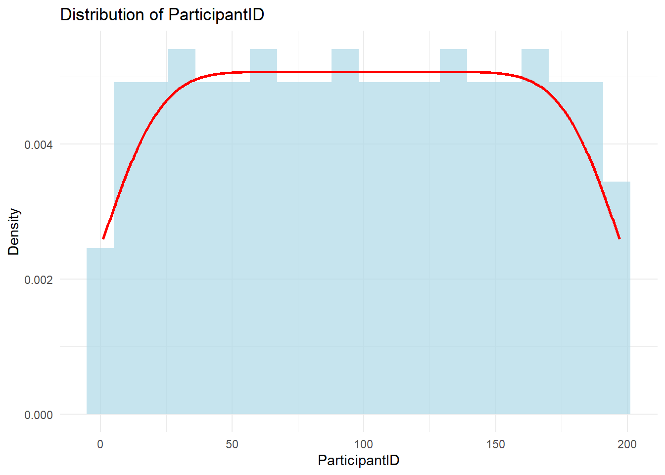
 $ ParticipantID        : num [1:197] 1 2 3 4 5 6 7 8 9 10 ...
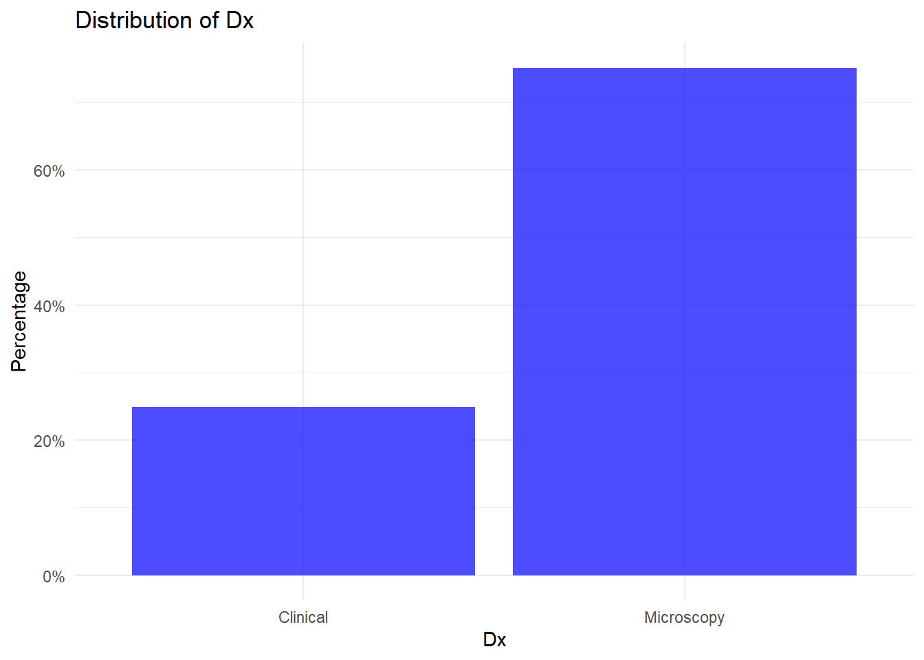
 $ Dx                   : chr [1:197] "Microscopy" "Clinical" "Microscopy" "Microscopy" ...
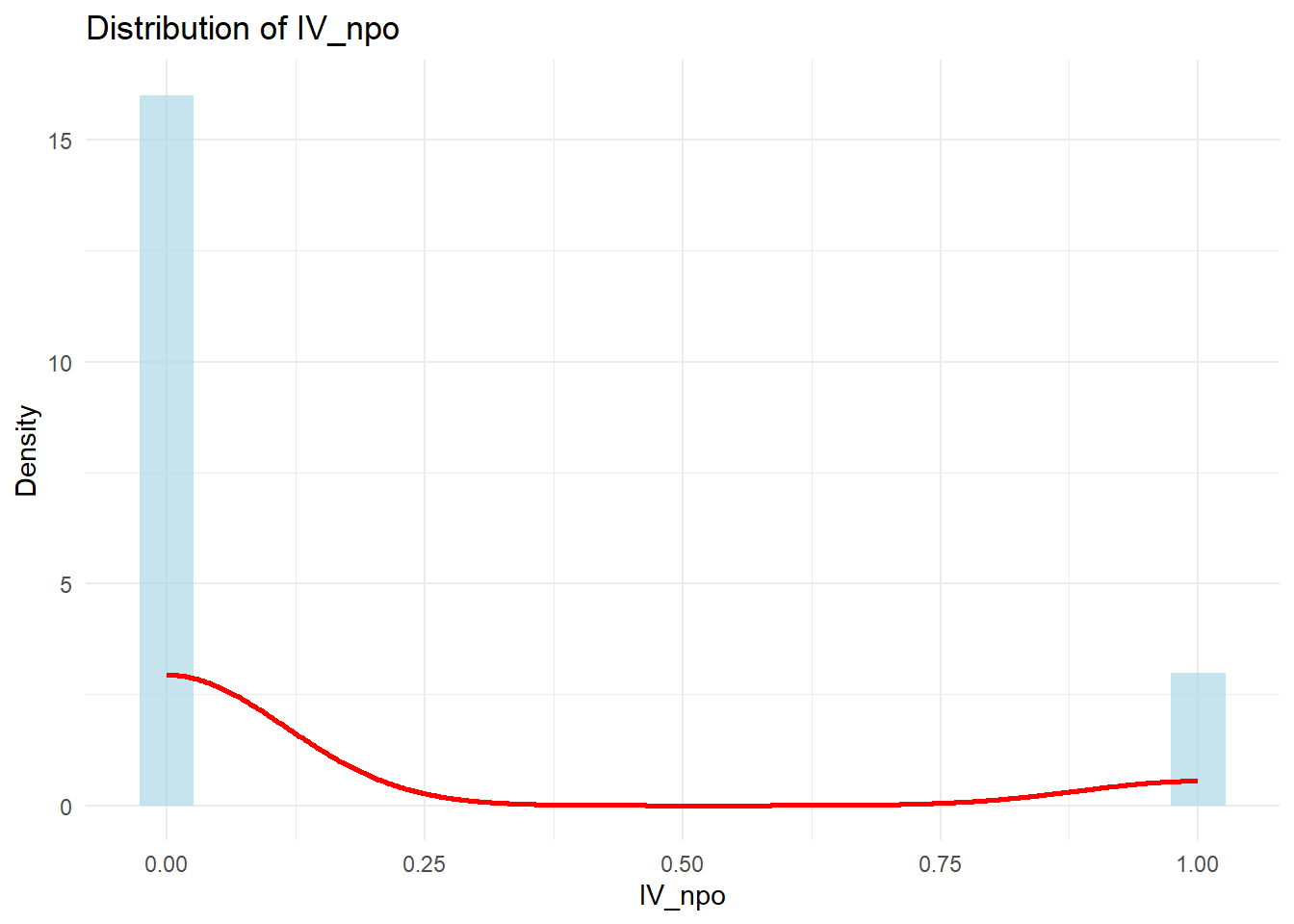
 $ IV_npo               : num [1:197] 0 0 0 0 1 1 0 0 1 0 ...
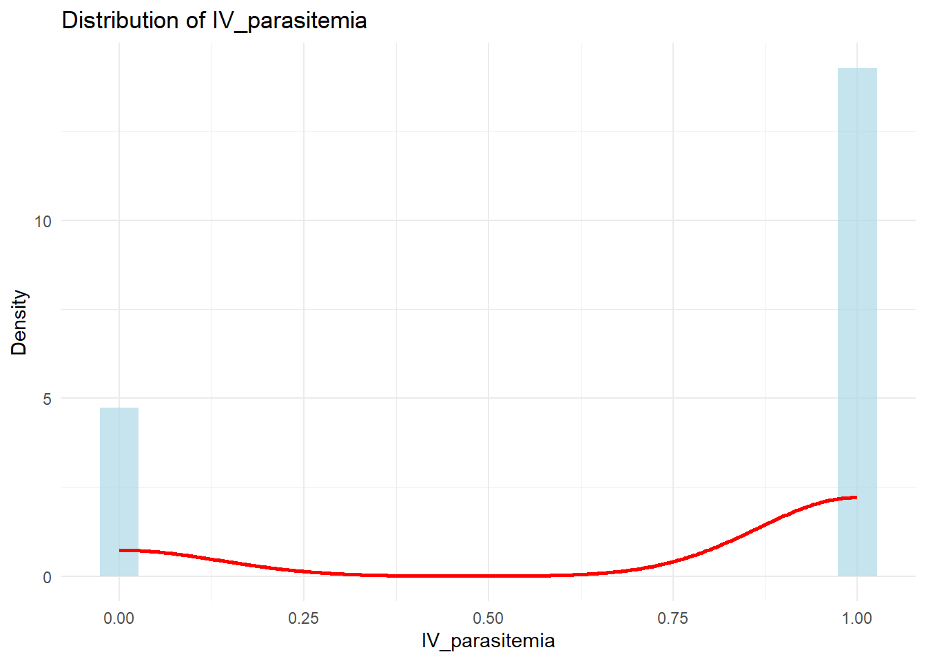
 $ IV_parasitemia       : num [1:197] 1 0 1 1 0 1 1 1 0 1 ...
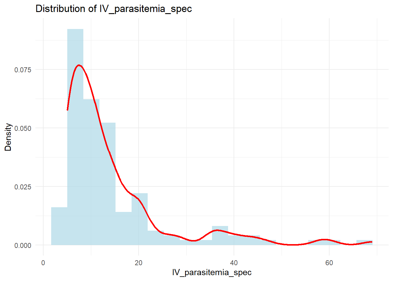
 $ IV_parasitemia_spec  : num [1:197] 11 NA 9.2 44 NA ...
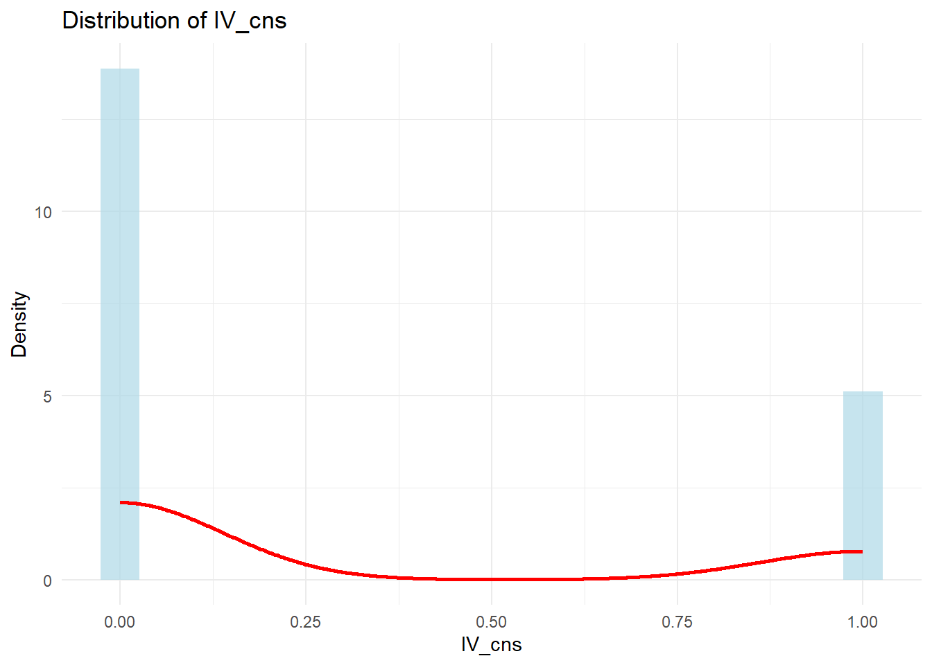
 $ IV_cns               : num [1:197] 1 0 0 1 1 0 0 0 0 0 ...
 $ IV_sz                : num [1:197] 0 0 0 0 0 0 0 0 0 0 ...
 $ IV_shock             : num [1:197] 0 0 0 1 0 0 0 0 1 0 ...
 $ IV_shock_pressors    : num [1:197] 0 0 0 1 0 0 0 0 1 0 ...
 $ IV_ards              : num [1:197] 0 0 0 0 0 0 0 0 0 0 ...
 $ IV_acidosis          : num [1:197] 0 0 0 0 0 0 0 0 0 0 ...
 $ IV_ARF               : num [1:197] 0 1 0 0 0 1 1 0 0 0 ...
 $ IV_ARF_BUN           : num [1:197] NA 56 NA NA NA 66 28 NA NA NA ...
 $ IV_ARF_creatinine    : num [1:197] NA 5 NA NA NA ...
 $ IV_DIC               : num [1:197] 0 1 0 0 0 0 0 0 0 0 ...
 $ IV_jaundice          : num [1:197] 0 1 0 0 0 1 1 0 0 0 ...
 $ IV_jaundice_bili     : num [1:197] NA 12.2 NA NA NA ...
 $ IV_anemia            : num [1:197] 0 0 0 0 0 0 0 0 1 0 ...
 $ IV_anemia_hgb        : num [1:197] NA NA NA NA NA ...
 $ Eligible             : num [1:197] 1 1 1 1 1 1 1 1 1 1 ...
 $ Severe               : num [1:197] 1 1 1 1 1 1 1 1 1 1 ...
 $ Date_consented       : chr [1:197] "04/06/2019 12:00:00 AM" "04/11/2019 12:00:00 AM" "04/13/2019 12:00:00 AM" "04/14/2019 12:00:00 AM" ...
 $ Date_recorded        : chr [1:197] "04/06/2019 12:00:00 AM" "04/11/2019 12:00:00 AM" "04/13/2019 12:00:00 AM" "04/15/2019 12:00:00 AM" ...
 $ Age Group            : chr [1:197] "19-60" "19-60" "5-18" "19-60" ...
 $ Sex                  : num [1:197] 0 0 1 1 1 1 1 0 1 0 ...
 $ Latino               : num [1:197] 0 0 0 0 0 0 0 0 0 0 ...
 $ Race                 : chr [1:197] "White" "Black/AA" "Black/AA" "Black/AA" ...
 $ Race_other_spec      : chr [1:197] NA NA NA NA ...
 $ Pregnant             : num [1:197] 0 0 0 0 0 0 0 0 0 0 ...
 $ EGA                  : num [1:197] NA NA NA NA NA NA NA NA NA NA ...
 $ Trimester            : num [1:197] NA NA NA NA NA NA NA NA NA NA ...
 $ Smear_done           : num [1:197] 1 1 1 1 1 1 1 1 1 1 ...
 $ Smear_read           : num [1:197] 1 1 1 1 1 1 1 1 1 1 ...
 $ Admit_species        : chr [1:197] "Pf" "Pf" "Pf" "Pf" ...
 $ Admit_mixed_specify  : chr [1:197] NA NA NA NA ...
 $ Admit_parasitemia    : num [1:197] 11 0.4 9.2 44 0.1 21 19.5 5.1 NA 7.4 ...
 $ Pre_antimalarial     : num [1:197] NA NA NA NA NA NA NA NA NA NA ...
 $ Pre_coartem          : num [1:197] NA NA NA NA NA NA NA NA NA NA ...
 $ Pre_malarone         : num [1:197] NA NA NA NA NA NA NA NA NA NA ...
 $ Pre_doxy             : num [1:197] NA NA NA NA NA NA NA NA NA NA ...
 $ Pre_mefloquine       : num [1:197] NA NA NA NA NA NA NA NA NA NA ...
 $ Pre_clinda           : num [1:197] NA NA NA NA NA NA NA NA NA NA ...
 $ Pre_quinine          : num [1:197] NA NA NA NA NA NA NA NA NA NA ...
 $ Pre_other            : num [1:197] NA NA NA NA NA NA NA NA NA NA ...
 $ Pre_other_spec       : logi [1:197] NA NA NA NA NA NA ...
 $ Admit_CBC_date       : chr [1:197] NA "04/09/2019 10:42:00 PM" "04/13/2019 01:33:00 PM" "04/14/2019 03:34:00 PM" ...
 $ Admit_CBC_time       : logi [1:197] FALSE TRUE TRUE TRUE FALSE TRUE ...
 $ Admit_HGB            : num [1:197] NA 15.7 10.9 10.5 11.3 9.5 12.5 10.5 6.7 14.9 ...
 $ Admit_HCT            : num [1:197] NA 46 33 34 32 30 37 31 19 45 ...
 $ Admit_PLT            : num [1:197] NA 72 176 43 133 46 14 57 44 44 ...
 $ Admit_WBC            : num [1:197] NA 7.8 6.5 4.03 8.01 ...
 $ Admit_chempanel_date : chr [1:197] NA "04/09/2019 10:42:00 PM" "04/13/2019 01:33:00 PM" "04/14/2019 03:34:00 PM" ...
 $ Admit_chempanel_time : logi [1:197] FALSE TRUE TRUE TRUE FALSE TRUE ...
 $ Admit_Na             : num [1:197] NA 131 127 133 130 142 134 133 134 137 ...
 $ Admit_K              : num [1:197] NA 2.8 3.4 3.7 4.3 ...
 $ Admit_Cl             : num [1:197] NA 92 97 101 94 11 98 100 102 101 ...
 $ Admit_HCO3           : num [1:197] NA 27 21 NA 2 11 17 23 19 29 ...
 $ Admit_BUN            : num [1:197] NA 26 13 16 19 66 28 10 24 15 ...
 $ Admit_creatinine     : num [1:197] NA 1.3 0.53 0.9 1.1 ...
 $ Admit_glucose        : num [1:197] NA 167 124 106 121 109 96 90 117 138 ...
 $ Admit_AST            : num [1:197] NA 269 30 36 55 60 142 32 326 52 ...
 $ Admit_ALT            : num [1:197] NA 140 16 17 40 36 122 13 110 49 ...
 $ Admit_bili           : num [1:197] NA 4.2 0.3 2.7 0.8 ...
 $ Admit_LDH_date       : chr [1:197] NA "04/10/2019 07:42:00 AM" "04/13/2019 01:33:00 PM" "04/14/2019 03:34:00 PM" ...
 $ Admit_LDH_time       : logi [1:197] FALSE TRUE TRUE TRUE FALSE TRUE ...
 $ Admit_LDH            : num [1:197] NA 1999 NA NA NA ...
 $ AS_lot               : chr [1:197] "AA241-1-10-01" "AA241-1-10-01" "AA241-1-10-01" "AA241-1-10-01" ...
 $ Weight               : num [1:197] 102 95 28 68 65 100 91 22 63 86 ...
 $ Num_AS_std           : num [1:197] 4 4 4 4 4 4 4 4 4 4 ...
 $ Extra_AS             : num [1:197] 0 0 0 0 0 0 0 0 0 0 ...
 $ Extra_AS_npo         : num [1:197] NA NA NA NA NA NA NA NA NA NA ...
 $ Extra_AS_parasitemia : num [1:197] NA NA NA NA NA NA NA NA NA NA ...
 $ Extra_AS_other       : num [1:197] NA NA NA NA NA NA NA NA NA NA ...
 $ Extra_AS_other_spec  : chr [1:197] NA NA NA NA ...
 $ FollowOn_oral        : num [1:197] 1 1 1 1 1 1 1 1 1 1 ...
 $ FollowOn_oral_spec   : chr [1:197] NA NA NA NA ...
 $ FollowOn_ok          : num [1:197] 1 1 1 1 1 1 1 1 1 1 ...
 $ FollowOn_notes       : chr [1:197] NA NA NA NA ...
 $ Adjunct_tx           : num [1:197] 0 1 0 1 0 1 1 0 0 0 ...
 $ Transfusion          : num [1:197] 0 0 0 0 0 1 1 0 0 0 ...
 $ Exchange             : num [1:197] 0 0 0 0 0 0 0 0 0 0 ...
 $ Dialysis             : num [1:197] 0 1 0 0 0 0 0 0 0 0 ...
 $ Vasopressors         : num [1:197] 0 0 0 1 0 0 0 0 0 0 ...
 $ Adjunct_other        : num [1:197] 0 0 0 0 0 1 0 0 0 0 ...
 $ Adjunct_other_spec   : chr [1:197] NA NA NA NA ...
 $ FU_CBC_date          : chr [1:197] NA "04/13/2019 02:49:00 PM" "04/16/2019 04:05:00 AM" "04/17/2019 05:50:00 AM" ...
 $ FU_CBC_time          : logi [1:197] FALSE TRUE TRUE TRUE TRUE TRUE ...
 $ FU_HGB               : num [1:197] NA 10.8 8.9 8.5 8.5 ...
 $ FU_HCT               : num [1:197] NA 30 27 27 26 21 27 27 23 43 ...
 $ FU_PLT               : num [1:197] NA 68 227 120 NA 51 5 152 107 101 ...
 $ FU_WBC               : num [1:197] NA 10.9 5.6 3.46 9.18 ...
 $ FU_chempanel_date    : chr [1:197] NA "04/13/2019 02:49:00 PM" "04/16/2019 04:05:00 AM" "04/17/2019 05:50:00 AM" ...
 $ FU_chempanel_time    : logi [1:197] FALSE TRUE TRUE TRUE TRUE TRUE ...
 $ FU_Na                : num [1:197] NA 132 135 139 135 153 129 137 140 142 ...
 $ FU_K                 : num [1:197] NA 3.4 3.9 3.6 4.1 ...
 $ FU_Cl                : num [1:197] NA 96 101 106 104 124 98 104 106 103 ...
 $ FU_HCO3              : num [1:197] NA 27 27 NA 23 25 20 27 23 29 ...
 $ FU_BUN               : num [1:197] NA 28 4 7 6 37 88 6 20 9 ...
 $ FU_creatinine        : num [1:197] NA 3.2 0.36 0.6 0.9 ...
  [list output truncated]
 - attr(*, "spec")=
  .. cols(
  ..   ParticipantID = col_double(),
  ..   Dx = col_character(),
  ..   IV_npo = col_double(),
  ..   IV_parasitemia = col_double(),
  ..   IV_parasitemia_spec = col_double(),
  ..   IV_cns = col_double(),
  ..   IV_sz = col_double(),
  ..   IV_shock = col_double(),
  ..   IV_shock_pressors = col_double(),
  ..   IV_ards = col_double(),
  ..   IV_acidosis = col_double(),
  ..   IV_ARF = col_double(),
  ..   IV_ARF_BUN = col_double(),
  ..   IV_ARF_creatinine = col_double(),
  ..   IV_DIC = col_double(),
  ..   IV_jaundice = col_double(),
  ..   IV_jaundice_bili = col_double(),
  ..   IV_anemia = col_double(),
  ..   IV_anemia_hgb = col_double(),
  ..   Eligible = col_double(),
  ..   Severe = col_double(),
  ..   Date_consented = col_character(),
  ..   Date_recorded = col_character(),
  ..   `Age Group` = col_character(),
  ..   Sex = col_double(),
  ..   Latino = col_double(),
  ..   Race = col_character(),
  ..   Race_other_spec = col_character(),
  ..   Pregnant = col_double(),
  ..   EGA = col_double(),
  ..   Trimester = col_double(),
  ..   Smear_done = col_double(),
  ..   Smear_read = col_double(),
  ..   Admit_species = col_character(),
  ..   Admit_mixed_specify = col_character(),
  ..   Admit_parasitemia = col_double(),
  ..   Pre_antimalarial = col_double(),
  ..   Pre_coartem = col_double(),
  ..   Pre_malarone = col_double(),
  ..   Pre_doxy = col_double(),
  ..   Pre_mefloquine = col_double(),
  ..   Pre_clinda = col_double(),
  ..   Pre_quinine = col_double(),
  ..   Pre_other = col_double(),
  ..   Pre_other_spec = col_logical(),
  ..   Admit_CBC_date = col_character(),
  ..   Admit_CBC_time = col_logical(),
  ..   Admit_HGB = col_double(),
  ..   Admit_HCT = col_double(),
  ..   Admit_PLT = col_double(),
  ..   Admit_WBC = col_double(),
  ..   Admit_chempanel_date = col_character(),
  ..   Admit_chempanel_time = col_logical(),
  ..   Admit_Na = col_double(),
  ..   Admit_K = col_double(),
  ..   Admit_Cl = col_double(),
  ..   Admit_HCO3 = col_double(),
  ..   Admit_BUN = col_double(),
  ..   Admit_creatinine = col_double(),
  ..   Admit_glucose = col_double(),
  ..   Admit_AST = col_double(),
  ..   Admit_ALT = col_double(),
  ..   Admit_bili = col_double(),
  ..   Admit_LDH_date = col_character(),
  ..   Admit_LDH_time = col_logical(),
  ..   Admit_LDH = col_double(),
  ..   AS_lot = col_character(),
  ..   Weight = col_double(),
  ..   Num_AS_std = col_double(),
  ..   Extra_AS = col_double(),
  ..   Extra_AS_npo = col_double(),
  ..   Extra_AS_parasitemia = col_double(),
  ..   Extra_AS_other = col_double(),
  ..   Extra_AS_other_spec = col_character(),
  ..   FollowOn_oral = col_double(),
  ..   FollowOn_oral_spec = col_character(),
  ..   FollowOn_ok = col_double(),
  ..   FollowOn_notes = col_character(),
  ..   Adjunct_tx = col_double(),
  ..   Transfusion = col_double(),
  ..   Exchange = col_double(),
  ..   Dialysis = col_double(),
  ..   Vasopressors = col_double(),
  ..   Adjunct_other = col_double(),
  ..   Adjunct_other_spec = col_character(),
  ..   FU_CBC_date = col_character(),
  ..   FU_CBC_time = col_logical(),
  ..   FU_HGB = col_double(),
  ..   FU_HCT = col_double(),
  ..   FU_PLT = col_double(),
  ..   FU_WBC = col_double(),
  ..   FU_chempanel_date = col_character(),
  ..   FU_chempanel_time = col_logical(),
  ..   FU_Na = col_double(),
  ..   FU_K = col_double(),
  ..   FU_Cl = col_double(),
  ..   FU_HCO3 = col_double(),
  ..   FU_BUN = col_double(),
  ..   FU_creatinine = col_double(),
  ..   FU_glucose = col_double(),
  ..   FU_AST = col_double(),
  ..   FU_ALT = col_double(),
  ..   FU_bili = col_double(),
  ..   FU_LDH_date = col_character(),
  ..   FU_LDH_time = col_logical(),
  ..   FU_LDH = col_double(),
  ..   End_date = col_character(),
  ..   Tx_complete = col_double(),
  ..   Incomplete_spec = col_character(),
  ..   Incomplete_other_spec = col_character(),
  ..   FO_coartem = col_double(),
  ..   FO_malarone = col_double(),
  ..   FO_doxy = col_double(),
  ..   FO_mefloquine = col_double(),
  ..   FO_clinda = col_double(),
  ..   FO_quinine = col_double(),
  ..   FO_other = col_double(),
  ..   FO_other_spec = col_logical(),
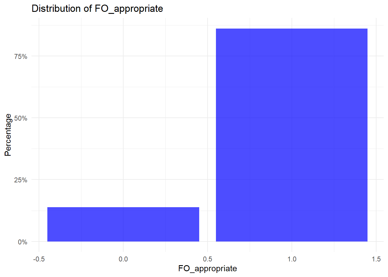
  ..   FO_appropriate = col_double()
  .. )
 - attr(*, "problems")=<externalptr>

# Summary statistics
summary(cdcMalaria)

 ParticipantID      Dx                IV_npo       IV_parasitemia  
 Min.   :  1   Length:197         Min.   :0.0000   Min.   :0.0000  
 1st Qu.: 50   Class :character   1st Qu.:0.0000   1st Qu.:1.0000  
 Median : 99   Mode  :character   Median :0.0000   Median :1.0000  
 Mean   : 99                      Mean   :0.1574   Mean   :0.7513  
 3rd Qu.:148                      3rd Qu.:0.0000   3rd Qu.:1.0000  
 Max.   :197                      Max.   :1.0000   Max.   :1.0000  
                                                                   
 IV_parasitemia_spec     IV_cns          IV_sz            IV_shock     
 Min.   : 5.00       Min.   :0.000   Min.   :0.00000   Min.   :0.0000  
 1st Qu.: 7.00       1st Qu.:0.000   1st Qu.:0.00000   1st Qu.:0.0000  
 Median :10.00       Median :0.000   Median :0.00000   Median :0.0000  
 Mean   :13.98       Mean   :0.269   Mean   :0.03553   Mean   :0.1523  
 3rd Qu.:15.18       3rd Qu.:1.000   3rd Qu.:0.00000   3rd Qu.:0.0000  
 Max.   :69.00       Max.   :1.000   Max.   :1.00000   Max.   :1.0000  
 NA's   :49                                                            
 IV_shock_pressors    IV_ards         IV_acidosis         IV_ARF      
 Min.   :0.0000    Min.   :0.00000   Min.   :0.0000   Min.   :0.0000  
 1st Qu.:0.0000    1st Qu.:0.00000   1st Qu.:0.0000   1st Qu.:0.0000  
 Median :0.0000    Median :0.00000   Median :0.0000   Median :0.0000  
 Mean   :0.1066    Mean   :0.08122   Mean   :0.2081   Mean   :0.3096  
 3rd Qu.:0.0000    3rd Qu.:0.00000   3rd Qu.:0.0000   3rd Qu.:1.0000  
 Max.   :1.0000    Max.   :1.00000   Max.   :1.0000   Max.   :1.0000  
                                                                      
   IV_ARF_BUN     IV_ARF_creatinine     IV_DIC         IV_jaundice    
 Min.   :  9.00   Min.   :0.500     Min.   :0.00000   Min.   :0.0000  
 1st Qu.: 21.00   1st Qu.:1.400     1st Qu.:0.00000   1st Qu.:0.0000  
 Median : 28.00   Median :2.190     Median :0.00000   Median :0.0000  
 Mean   : 38.44   Mean   :2.382     Mean   :0.09137   Mean   :0.3046  
 3rd Qu.: 51.00   3rd Qu.:2.900     3rd Qu.:0.00000   3rd Qu.:1.0000  
 Max.   :125.00   Max.   :7.100     Max.   :1.00000   Max.   :1.0000  
 NA's   :138      NA's   :136                                         
 IV_jaundice_bili   IV_anemia       IV_anemia_hgb      Eligible
 Min.   : 1.100   Min.   :0.00000   Min.   :3.700   Min.   :1  
 1st Qu.: 2.900   1st Qu.:0.00000   1st Qu.:5.750   1st Qu.:1  
 Median : 4.100   Median :0.00000   Median :6.400   Median :1  
 Mean   : 5.957   Mean   :0.09645   Mean   :6.147   Mean   :1  
 3rd Qu.: 7.725   3rd Qu.:0.00000   3rd Qu.:6.700   3rd Qu.:1  
 Max.   :23.700   Max.   :1.00000   Max.   :6.900   Max.   :1  
 NA's   :137                        NA's   :178                
     Severe       Date_consented     Date_recorded       Age Group        
 Min.   :0.0000   Length:197         Length:197         Length:197        
 1st Qu.:1.0000   Class :character   Class :character   Class :character  
 Median :1.0000   Mode  :character   Mode  :character   Mode  :character  
 Mean   :0.9848                                                           
 3rd Qu.:1.0000                                                           
 Max.   :1.0000                                                           
                                                                          
      Sex            Latino            Race           Race_other_spec   
 Min.   :0.000   Min.   :0.00000   Length:197         Length:197        
 1st Qu.:0.000   1st Qu.:0.00000   Class :character   Class :character  
 Median :0.000   Median :0.00000   Mode  :character   Mode  :character  
 Mean   :0.401   Mean   :0.01531                                        
 3rd Qu.:1.000   3rd Qu.:0.00000                                        
 Max.   :1.000   Max.   :1.00000                                        
                 NA's   :1                                              
    Pregnant            EGA          Trimester     Smear_done   Smear_read    
 Min.   :0.00000   Min.   :28.00   Min.   :3     Min.   :1    Min.   :0.0000  
 1st Qu.:0.00000   1st Qu.:28.75   1st Qu.:3     1st Qu.:1    1st Qu.:1.0000  
 Median :0.00000   Median :29.50   Median :3     Median :1    Median :1.0000  
 Mean   :0.01015   Mean   :29.50   Mean   :3     Mean   :1    Mean   :0.9949  
 3rd Qu.:0.00000   3rd Qu.:30.25   3rd Qu.:3     3rd Qu.:1    3rd Qu.:1.0000  
 Max.   :1.00000   Max.   :31.00   Max.   :3     Max.   :1    Max.   :1.0000  
                   NA's   :195     NA's   :195                                
 Admit_species      Admit_mixed_specify Admit_parasitemia Pre_antimalarial
 Length:197         Length:197          Min.   : 0.10     Min.   :0.0000  
 Class :character   Class :character    1st Qu.: 4.30     1st Qu.:1.0000  
 Mode  :character   Mode  :character    Median : 8.00     Median :1.0000  
                                        Mean   :10.87     Mean   :0.9487  
                                        3rd Qu.:13.60     3rd Qu.:1.0000  
                                        Max.   :69.00     Max.   :1.0000  
                                        NA's   :2         NA's   :158     
  Pre_coartem      Pre_malarone       Pre_doxy      Pre_mefloquine   
 Min.   :0.0000   Min.   :0.0000   Min.   :0.0000   Min.   :0.00000  
 1st Qu.:0.0000   1st Qu.:0.0000   1st Qu.:0.0000   1st Qu.:0.00000  
 Median :0.0000   Median :0.0000   Median :0.0000   Median :0.00000  
 Mean   :0.3846   Mean   :0.4615   Mean   :0.1026   Mean   :0.05128  
 3rd Qu.:1.0000   3rd Qu.:1.0000   3rd Qu.:0.0000   3rd Qu.:0.00000  
 Max.   :1.0000   Max.   :1.0000   Max.   :1.0000   Max.   :1.00000  
 NA's   :158      NA's   :158      NA's   :158      NA's   :158      
   Pre_clinda       Pre_quinine        Pre_other   Pre_other_spec
 Min.   :0.00000   Min.   :0.00000   Min.   :0     Mode:logical  
 1st Qu.:0.00000   1st Qu.:0.00000   1st Qu.:0     NA's:197      
 Median :0.00000   Median :0.00000   Median :0                   
 Mean   :0.02564   Mean   :0.07895   Mean   :0                   
 3rd Qu.:0.00000   3rd Qu.:0.00000   3rd Qu.:0                   
 Max.   :1.00000   Max.   :1.00000   Max.   :0                   
 NA's   :158       NA's   :159       NA's   :158                 
 Admit_CBC_date     Admit_CBC_time    Admit_HGB       Admit_HCT    
 Length:197         Mode :logical   Min.   : 3.70   Min.   :11.00  
 Class :character   FALSE:14        1st Qu.: 9.90   1st Qu.:30.00  
 Mode  :character   TRUE :183       Median :11.80   Median :35.00  
                                    Mean   :11.49   Mean   :34.36  
                                    3rd Qu.:13.38   3rd Qu.:39.00  
                                    Max.   :17.00   Max.   :49.00  
                                    NA's   :3       NA's   :4      
   Admit_PLT        Admit_WBC      Admit_chempanel_date Admit_chempanel_time
 Min.   :  4.00   Min.   : 1.380   Length:197           Mode :logical       
 1st Qu.: 32.00   1st Qu.: 4.463   Class :character     FALSE:13            
 Median : 50.00   Median : 6.135   Mode  :character     TRUE :184           
 Mean   : 68.56   Mean   : 6.842                                            
 3rd Qu.: 89.25   3rd Qu.: 8.018                                            
 Max.   :254.00   Max.   :31.800                                            
 NA's   :5        NA's   :3                                                 
    Admit_Na        Admit_K         Admit_Cl        Admit_HCO3   
 Min.   :116.0   Min.   :2.300   Min.   : 11.00   Min.   : 2.00  
 1st Qu.:131.0   1st Qu.:3.500   1st Qu.: 96.00   1st Qu.:19.00  
 Median :134.0   Median :3.800   Median :101.00   Median :22.00  
 Mean   :133.9   Mean   :3.876   Mean   : 99.35   Mean   :20.95  
 3rd Qu.:137.0   3rd Qu.:4.200   3rd Qu.:105.00   3rd Qu.:23.00  
 Max.   :153.0   Max.   :6.900   Max.   :123.00   Max.   :29.00  
 NA's   :3       NA's   :3       NA's   :4        NA's   :14     
   Admit_BUN     Admit_creatinine Admit_glucose     Admit_AST     
 Min.   : 3.00   Min.   :0.230    Min.   : 11.0   Min.   : 14.00  
 1st Qu.:13.00   1st Qu.:0.700    1st Qu.: 95.0   1st Qu.: 37.00  
 Median :18.00   Median :1.045    Median :107.0   Median : 54.00  
 Mean   :22.99   Mean   :1.295    Mean   :120.8   Mean   : 80.66  
 3rd Qu.:26.75   3rd Qu.:1.515    3rd Qu.:126.5   3rd Qu.: 93.25  
 Max.   :87.00   Max.   :6.560    Max.   :398.0   Max.   :903.00  
 NA's   :7       NA's   :3        NA's   :6       NA's   :5       
   Admit_ALT        Admit_bili     Admit_LDH_date     Admit_LDH_time 
 Min.   :  5.00   Min.   : 0.300   Length:197         Mode :logical  
 1st Qu.: 24.00   1st Qu.: 1.192   Class :character   FALSE:13       
 Median : 39.00   Median : 2.100   Mode  :character   TRUE :184      
 Mean   : 57.81   Mean   : 3.245                                     
 3rd Qu.: 74.00   3rd Qu.: 3.925                                     
 Max.   :364.00   Max.   :23.700                                     
 NA's   :4        NA's   :5                                          
   Admit_LDH          AS_lot              Weight         Num_AS_std   
 Min.   :    3.0   Length:197         Min.   :  9.20   Min.   :3.000  
 1st Qu.:  369.5   Class :character   1st Qu.: 52.00   1st Qu.:4.000  
 Median :  564.0   Mode  :character   Median : 73.00   Median :4.000  
 Mean   :  861.5                      Mean   : 68.59   Mean   :3.792  
 3rd Qu.:  892.5                      3rd Qu.: 88.00   3rd Qu.:4.000  
 Max.   :11572.0                      Max.   :153.00   Max.   :4.000  
 NA's   :101                                                          
    Extra_AS        Extra_AS_npo Extra_AS_parasitemia Extra_AS_other  
 Min.   :0.00000   Min.   :0     Min.   :0.0000       Min.   :0.0000  
 1st Qu.:0.00000   1st Qu.:0     1st Qu.:0.0000       1st Qu.:0.0000  
 Median :0.00000   Median :0     Median :0.0000       Median :1.0000  
 Mean   :0.03046   Mean   :0     Mean   :0.2857       Mean   :0.5714  
 3rd Qu.:0.00000   3rd Qu.:0     3rd Qu.:0.5000       3rd Qu.:1.0000  
 Max.   :1.00000   Max.   :0     Max.   :1.0000       Max.   :1.0000  
                   NA's   :190   NA's   :190          NA's   :190     
 Extra_AS_other_spec FollowOn_oral    FollowOn_oral_spec  FollowOn_ok    
 Length:197          Min.   :0.0000   Length:197         Min.   :0.0000  
 Class :character    1st Qu.:1.0000   Class :character   1st Qu.:1.0000  
 Mode  :character    Median :1.0000   Mode  :character   Median :1.0000  
                     Mean   :0.9391                      Mean   :0.9615  
                     3rd Qu.:1.0000                      3rd Qu.:1.0000  
                     Max.   :1.0000                      Max.   :1.0000  
                                                         NA's   :15      
 FollowOn_notes       Adjunct_tx      Transfusion        Exchange      
 Length:197         Min.   :0.0000   Min.   :0.0000   Min.   :0.00000  
 Class :character   1st Qu.:0.0000   1st Qu.:0.0000   1st Qu.:0.00000  
 Mode  :character   Median :0.0000   Median :0.0000   Median :0.00000  
                    Mean   :0.4112   Mean   :0.2437   Mean   :0.01523  
                    3rd Qu.:1.0000   3rd Qu.:0.0000   3rd Qu.:0.00000  
                    Max.   :1.0000   Max.   :1.0000   Max.   :1.00000  
                                                                       
    Dialysis        Vasopressors    Adjunct_other    Adjunct_other_spec
 Min.   :0.00000   Min.   :0.0000   Min.   :0.0000   Length:197        
 1st Qu.:0.00000   1st Qu.:0.0000   1st Qu.:0.0000   Class :character  
 Median :0.00000   Median :0.0000   Median :0.0000   Mode  :character  
 Mean   :0.07614   Mean   :0.1218   Mean   :0.1472                     
 3rd Qu.:0.00000   3rd Qu.:0.0000   3rd Qu.:0.0000                     
 Max.   :1.00000   Max.   :1.0000   Max.   :1.0000                     
                                                                       
 FU_CBC_date        FU_CBC_time         FU_HGB           FU_HCT     
 Length:197         Mode :logical   Min.   : 3.800   Min.   : 9.00  
 Class :character   FALSE:11        1st Qu.: 8.500   1st Qu.:25.25  
 Mode  :character   TRUE :186       Median : 9.500   Median :28.00  
                                    Mean   : 9.563   Mean   :28.36  
                                    3rd Qu.:10.875   3rd Qu.:33.00  
                                    Max.   :13.800   Max.   :43.00  
                                    NA's   :7        NA's   :7      
     FU_PLT           FU_WBC       FU_chempanel_date  FU_chempanel_time
 Min.   :  4.00   Min.   : 1.460   Length:197         Mode :logical    
 1st Qu.: 54.25   1st Qu.: 4.900   Class :character   FALSE:11         
 Median : 88.50   Median : 6.100   Mode  :character   TRUE :186        
 Mean   : 94.81   Mean   : 7.226                                       
 3rd Qu.:127.75   3rd Qu.: 8.450                                       
 Max.   :254.00   Max.   :27.100                                       
 NA's   :7        NA's   :6                                            
     FU_Na          FU_K           FU_Cl          FU_HCO3         FU_BUN     
 Min.   :126   Min.   :2.600   Min.   : 90.0   Min.   : 0.0   Min.   : 3.00  
 1st Qu.:135   1st Qu.:3.600   1st Qu.:102.0   1st Qu.:21.0   1st Qu.: 8.00  
 Median :137   Median :3.800   Median :105.0   Median :23.0   Median :12.00  
 Mean   :137   Mean   :3.892   Mean   :105.3   Mean   :22.8   Mean   :17.93  
 3rd Qu.:139   3rd Qu.:4.100   3rd Qu.:108.0   3rd Qu.:25.0   3rd Qu.:19.00  
 Max.   :155   Max.   :6.500   Max.   :128.0   Max.   :30.0   Max.   :88.00  
 NA's   :6     NA's   :6       NA's   :6       NA's   :16     NA's   :9      
 FU_creatinine     FU_glucose        FU_AST           FU_ALT      
 Min.   :0.190   Min.   : 12.0   Min.   :  15.0   Min.   :  7.00  
 1st Qu.:0.540   1st Qu.: 90.0   1st Qu.:  42.0   1st Qu.: 27.00  
 Median :0.790   Median : 99.5   Median :  79.0   Median : 48.00  
 Mean   :1.256   Mean   :105.3   Mean   : 105.6   Mean   : 69.56  
 3rd Qu.:1.090   3rd Qu.:115.2   3rd Qu.: 130.0   3rd Qu.: 91.00  
 Max.   :6.730   Max.   :322.0   Max.   :1817.0   Max.   :688.00  
 NA's   :6       NA's   :9       NA's   :26       NA's   :26      
    FU_bili       FU_LDH_date        FU_LDH_time         FU_LDH       
 Min.   : 0.020   Length:197         Mode :logical   Min.   :    3.0  
 1st Qu.: 0.530   Class :character   FALSE:27        1st Qu.:  412.0  
 Median : 1.000   Mode  :character   TRUE :170       Median :  659.0  
 Mean   : 2.412                                      Mean   :  939.7  
 3rd Qu.: 2.400                                      3rd Qu.:  959.0  
 Max.   :21.700                                      Max.   :14930.0  
 NA's   :29                                          NA's   :118      
   End_date          Tx_complete     Incomplete_spec    Incomplete_other_spec
 Length:197         Min.   :0.0000   Length:197         Length:197           
 Class :character   1st Qu.:1.0000   Class :character   Class :character     
 Mode  :character   Median :1.0000   Mode  :character   Mode  :character     
                    Mean   :0.9543                                           
                    3rd Qu.:1.0000                                           
                    Max.   :1.0000                                           
                                                                             
   FO_coartem      FO_malarone        FO_doxy        FO_mefloquine     
 Min.   :0.0000   Min.   :0.0000   Min.   :0.00000   Min.   :0.000000  
 1st Qu.:0.0000   1st Qu.:0.0000   1st Qu.:0.00000   1st Qu.:0.000000  
 Median :0.0000   Median :1.0000   Median :0.00000   Median :0.000000  
 Mean   :0.2887   Mean   :0.5515   Mean   :0.08247   Mean   :0.005155  
 3rd Qu.:1.0000   3rd Qu.:1.0000   3rd Qu.:0.00000   3rd Qu.:0.000000  
 Max.   :1.0000   Max.   :1.0000   Max.   :1.00000   Max.   :1.000000  
 NA's   :3        NA's   :3        NA's   :3         NA's   :3         
   FO_clinda         FO_quinine         FO_other FO_other_spec 
 Min.   :0.00000   Min.   :0.00000   Min.   :0   Mode:logical  
 1st Qu.:0.00000   1st Qu.:0.00000   1st Qu.:0   NA's:197      
 Median :0.00000   Median :0.00000   Median :0                 
 Mean   :0.03093   Mean   :0.01036   Mean   :0                 
 3rd Qu.:0.00000   3rd Qu.:0.00000   3rd Qu.:0                 
 Max.   :1.00000   Max.   :1.00000   Max.   :0                 
 NA's   :3         NA's   :4         NA's   :4                 
 FO_appropriate  
 Min.   :0.0000  
 1st Qu.:1.0000  
 Median :1.0000  
 Mean   :0.8619  
 3rd Qu.:1.0000  
 Max.   :1.0000  
 NA's   :16

Summary Tables

# Selecting categorical variables/Distribution of Categorical Variables %
categorical_vars <- c("Dx", "FO_appropriate")

# Function to compute percentage distribution
categorical_summary <- function(df, var) {
  df %>%
    group_by(.data[[var]]) %>%
    summarise(Count = n(), Percentage = (n() / nrow(df)) * 100)
}

# Computing summary for each categorical variable
cat_summary_list <- lapply(categorical_vars, function(var) categorical_summary(cdcMalaria, var))

# Printing categorical summaries
cat_summary_list

[[1]]
# A tibble: 2 × 3
  Dx         Count Percentage
  <chr>      <int>      <dbl>
1 Clinical      49       24.9
2 Microscopy   148       75.1

[[2]]
# A tibble: 3 × 3
  FO_appropriate Count Percentage
           <dbl> <int>      <dbl>
1              0    25      12.7 
2              1   156      79.2 
3             NA    16       8.12

Summary Statistics for Continuous Variables

# Selecting continuous variables
# Summary Statistics for Continuous Variables with Missing Value Handling
continuous_vars <- cdcMalaria %>%
  select(where(is.numeric)) %>%
  summarise_all(list(
    mean = ~mean(., na.rm = TRUE),
    sd = ~sd(., na.rm = TRUE),
    min = ~min(., na.rm = TRUE),
    q25 = ~quantile(., 0.25, na.rm = TRUE),
    median = ~median(., na.rm = TRUE),
    q75 = ~quantile(., 0.75, na.rm = TRUE),
    max = ~max(., na.rm = TRUE)
  ))

# Printing summary table
print(continuous_vars)

# A tibble: 1 × 623
  ParticipantID_mean IV_npo_mean IV_parasitemia_mean IV_parasitemia_spec_mean
               <dbl>       <dbl>               <dbl>                    <dbl>
1                 99       0.157               0.751                     14.0
# ℹ 619 more variables: IV_cns_mean <dbl>, IV_sz_mean <dbl>,
#   IV_shock_mean <dbl>, IV_shock_pressors_mean <dbl>, IV_ards_mean <dbl>,
#   IV_acidosis_mean <dbl>, IV_ARF_mean <dbl>, IV_ARF_BUN_mean <dbl>,
#   IV_ARF_creatinine_mean <dbl>, IV_DIC_mean <dbl>, IV_jaundice_mean <dbl>,
#   IV_jaundice_bili_mean <dbl>, IV_anemia_mean <dbl>,
#   IV_anemia_hgb_mean <dbl>, Eligible_mean <dbl>, Severe_mean <dbl>,
#   Sex_mean <dbl>, Latino_mean <dbl>, Pregnant_mean <dbl>, EGA_mean <dbl>, …

Visualizations/Bar Charts for Categorical Variables

# Function to plot categorical variable distribution
plot_categorical <- function(df, var) {
  ggplot(df, aes(x = .data[[var]])) +
    geom_bar(aes(y = (..count..) / sum(..count..)), fill = "blue", alpha = 0.7) +
    scale_y_continuous(labels = scales::percent_format()) +
    labs(title = paste("Distribution of", var), y = "Percentage", x = var) +
    theme_minimal()
}

# Generating bar charts
for (var in categorical_vars) {
  print(plot_categorical(cdcMalaria, var))
}

Warning: The dot-dot notation (`..count..`) was deprecated in ggplot2 3.4.0.
ℹ Please use `after_stat(count)` instead.

Warning: Removed 16 rows containing non-finite outside the scale range
(`stat_count()`).

Histograms for Continuous Variables

# Function to plot histogram and density curve
plot_histogram <- function(df, var) {
  ggplot(df, aes(x = .data[[var]])) +
    geom_histogram(aes(y = ..density..), bins = 20, fill = "lightblue", alpha = 0.7) +
    geom_density(color = "red", size = 1) +
    labs(title = paste("Distribution of", var), x = var, y = "Density") +
    theme_minimal()
}

# Select numeric variables from the original dataset
numeric_vars <- names(cdcMalaria %>% select(where(is.numeric)))

# Plot first 5 continuous variables
for (var in numeric_vars[1:5]) {  # Use column names from the original dataset
  print(plot_histogram(cdcMalaria, var))
}

Warning: Using `size` aesthetic for lines was deprecated in ggplot2 3.4.0.
ℹ Please use `linewidth` instead.

Warning: Removed 49 rows containing non-finite outside the scale range
(`stat_bin()`).

Warning: Removed 49 rows containing non-finite outside the scale range
(`stat_density()`).

This part was contributed by Murtaza Yaqubi.

It’s a good practice to install and load the necessary packages for analysis.

library(dplyr)
library(tidyverse)

Warning: package 'tidyverse' was built under R version 4.4.2

Warning: package 'purrr' was built under R version 4.4.2

Warning: package 'lubridate' was built under R version 4.4.2

── Attaching core tidyverse packages ──────────────────────── tidyverse 2.0.0 ──
✔ forcats   1.0.0     ✔ stringr   1.5.1
✔ lubridate 1.9.4     ✔ tibble    3.2.1
✔ purrr     1.0.4     
── Conflicts ────────────────────────────────────────── tidyverse_conflicts() ──
✖ tidyr::expand()  masks Matrix::expand()
✖ dplyr::filter()  masks stats::filter()
✖ purrr::flatten() masks jsonlite::flatten()
✖ dplyr::lag()     masks stats::lag()
✖ tidyr::pack()    masks Matrix::pack()
✖ tidyr::unpack()  masks Matrix::unpack()
ℹ Use the conflicted package (<http://conflicted.r-lib.org/>) to force all conflicts to become errors

library(ggplot2)

Generating synthetic data frame.

I created a synthetic data frame to replicate the analysis of the dataset above. To achieve this, I used the results of the original analysis to attempt to replicate the original dataset with its corresponding results. I began by setting a seed for reproducibility. Next, I defined the number of observations before introducing the codes for the variables in the data frame. The data frame contains two categorical variables and five continuous variables. These variables are Patient_ID, Condition, TreatmentGiven, BreathCount, Fever, Tachycardia, and Hypoglycemia.

# Set seed for reproducibility
set.seed(123)

# Define number of observations
n <- 197

# Generate synthetic dataset
HealthSynthetic <- data.frame(
  # Unique Patient ID
  Patient_ID = 1:n,
  
  # Categorical Variables (pneumonia and bronchitis)
  Condition = sample(c("Pneumonia", "Bronchitis"), n, replace = TRUE, prob = c(0.2487, 0.7513)),
  
  TreatmentGiven = sample(c(0, 1, NA), n, replace = TRUE, prob = c(0.1269, 0.7919, 0.0812)),
  
  # Continuous Variables (breath count, fever, tachycardia, hypoglycemia)
  BreathCount = round(rnorm(n, mean = 13.98141, sd = 11.31289)),
  
  Fever = sample(c(0, 1, NA), n, replace = TRUE, prob = c(0.90, 0.05, 0.05)), 
  
  Tachycardia = sample(c(0, 1, NA), n, replace = TRUE, prob = c(0.50, 0.45, 0.05)),  
  
  Hypoglycemia = sample(c(0, 1, NA), n, replace = TRUE, prob = c(0.75, 0.20, 0.05))  
)

# View the first few rows
head(HealthSynthetic)

  Patient_ID  Condition TreatmentGiven BreathCount Fever Tachycardia
1          1 Bronchitis              1           0     0           1
2          2  Pneumonia              1           7    NA           0
3          3 Bronchitis              1           1    NA           0
4          4  Pneumonia              1          39     0           0
5          5  Pneumonia             NA          29     0           0
6          6 Bronchitis              1          11     0           0
  Hypoglycemia
1            0
2            1
3            1
4            0
5            0
6            1

# Summary statistics
summary(HealthSynthetic)

   Patient_ID   Condition         TreatmentGiven    BreathCount    
 Min.   :  1   Length:197         Min.   :0.0000   Min.   :-14.00  
 1st Qu.: 50   Class :character   1st Qu.:1.0000   1st Qu.:  7.00  
 Median : 99   Mode  :character   Median :1.0000   Median : 14.00  
 Mean   : 99                      Mean   :0.8833   Mean   : 14.34  
 3rd Qu.:148                      3rd Qu.:1.0000   3rd Qu.: 22.00  
 Max.   :197                      Max.   :1.0000   Max.   : 43.00  
                                  NA's   :17                       
     Fever          Tachycardia      Hypoglycemia   
 Min.   :0.00000   Min.   :0.0000   Min.   :0.0000  
 1st Qu.:0.00000   1st Qu.:0.0000   1st Qu.:0.0000  
 Median :0.00000   Median :0.0000   Median :0.0000  
 Mean   :0.04839   Mean   :0.4607   Mean   :0.1809  
 3rd Qu.:0.00000   3rd Qu.:1.0000   3rd Qu.:0.0000  
 Max.   :1.00000   Max.   :1.0000   Max.   :1.0000  
 NA's   :11        NA's   :6        NA's   :9

# Check structure
str(HealthSynthetic)

'data.frame':   197 obs. of  7 variables:
 $ Patient_ID    : int  1 2 3 4 5 6 7 8 9 10 ...
 $ Condition     : chr  "Bronchitis" "Pneumonia" "Bronchitis" "Pneumonia" ...
 $ TreatmentGiven: num  1 1 1 1 NA 1 1 1 0 1 ...
 $ BreathCount   : num  0 7 1 39 29 11 20 9 9 5 ...
 $ Fever         : num  0 NA NA 0 0 0 0 0 0 0 ...
 $ Tachycardia   : num  1 0 0 0 0 0 0 1 0 1 ...
 $ Hypoglycemia  : num  0 1 1 0 0 1 0 0 0 0 ...

Summary statistics:

I generated the summary statistics for both categorical and continuous variables by leveraging loop functions. This approach allowed me to efficiently apply the same set of operations to multiple variables without repeating large chunks of code, thus streamlining the analysis process and minimizing the risk of errors.

library(tidyverse)

# Before producing summary tables, I have to convert "Condition" and "TreatmentGiven" to factors from characters.   
HealthSynthetic <- HealthSynthetic %>% 
  mutate(Condition = as.factor(Condition), TreatmentGiven = as.factor(TreatmentGiven))

# Categorical Variables Summary
categorical_vars <- c("Condition", "TreatmentGiven")

categorical_summary <- function(df, var) {
  df %>%
    group_by(.data[[var]]) %>%
    summarise(Count = n(), Percentage = (n() / nrow(df)) * 100)
}

# Compute summaries for categorical variables
cat_summary_list <- lapply(categorical_vars, function(var) categorical_summary(HealthSynthetic, var))

# Print categorical summaries
names(cat_summary_list) <- categorical_vars
print(cat_summary_list)

$Condition
# A tibble: 2 × 3
  Condition  Count Percentage
  <fct>      <int>      <dbl>
1 Bronchitis   150       76.1
2 Pneumonia     47       23.9

$TreatmentGiven
# A tibble: 3 × 3
  TreatmentGiven Count Percentage
  <fct>          <int>      <dbl>
1 0                 21      10.7 
2 1                159      80.7 
3 <NA>              17       8.63

# Continuous Variables Summary
continuous_vars <- c("Patient_ID", "BreathCount", "Fever", "Tachycardia", "Hypoglycemia")

continuous_summary <- HealthSynthetic %>%
  select(where(is.numeric)) %>%  # Select only numeric variables
  summarise_all(list(
    mean = ~mean(., na.rm = TRUE),
    sd = ~sd(., na.rm = TRUE),
    min = ~min(., na.rm = TRUE),
    q25 = ~quantile(., 0.25, na.rm = TRUE),
    median = ~median(., na.rm = TRUE),
    q75 = ~quantile(., 0.75, na.rm = TRUE),
    max = ~max(., na.rm = TRUE)
  ))

# Print continuous summary
print(continuous_summary)

  Patient_ID_mean BreathCount_mean Fever_mean Tachycardia_mean
1              99          14.3401  0.0483871         0.460733
  Hypoglycemia_mean Patient_ID_sd BreathCount_sd Fever_sd Tachycardia_sd
1         0.1808511      57.01316       11.30789 0.215162      0.4997657
  Hypoglycemia_sd Patient_ID_min BreathCount_min Fever_min Tachycardia_min
1       0.3859225              1             -14         0               0
  Hypoglycemia_min Patient_ID_q25 BreathCount_q25 Fever_q25 Tachycardia_q25
1                0             50               7         0               0
  Hypoglycemia_q25 Patient_ID_median BreathCount_median Fever_median
1                0                99                 14            0
  Tachycardia_median Hypoglycemia_median Patient_ID_q75 BreathCount_q75
1                  0                   0            148              22
  Fever_q75 Tachycardia_q75 Hypoglycemia_q75 Patient_ID_max BreathCount_max
1         0               1                0            197              43
  Fever_max Tachycardia_max Hypoglycemia_max
1         1               1                1

Plotting the data:

I used loop functions to generate bar plots for both categorical and continuous variables, enabling me to efficiently apply the same plotting logic to multiple variables without duplicating code. This approach streamlined the visualization process and made the code more compact and manageable.

# Function to plot categorical variable distribution
plot_categorical <- function(df, var) {
  ggplot(df, aes(x = as.factor(.data[[var]]))) +
    geom_bar(aes(y = (..count..) / sum(..count..)), fill = "purple", alpha = 0.8) +
    scale_y_continuous(labels = scales::percent_format()) +
    labs(title = paste("Distribution of", var), y = "Percentage", x = var) +
    theme_minimal()
}

# Categorical variables
categorical_vars <- c("Condition", "TreatmentGiven")

# Generating bar charts
for (var in categorical_vars) {
  print(plot_categorical(HealthSynthetic, var))
}

# Function to plot histogram and density curve
plot_histogram <- function(df, var) {
  ggplot(df, aes(x = .data[[var]])) +
    geom_histogram(aes(y = ..density..), bins = 20, fill = "steelblue", alpha = 0.7) +
    geom_density(color = "orange", size = 1) +
    labs(title = paste("Distribution of", var), x = var, y = "Density") +
    theme_minimal()
}

# Continuous variables
numeric_vars <- names(HealthSynthetic %>% select(where(is.numeric)))


# Plot continuous variables
for (var in numeric_vars) {  
  print(plot_histogram(HealthSynthetic, var))
}

Warning: Removed 11 rows containing non-finite outside the scale range
(`stat_bin()`).

Warning: Removed 11 rows containing non-finite outside the scale range
(`stat_density()`).

Warning: Removed 6 rows containing non-finite outside the scale range
(`stat_bin()`).

Warning: Removed 6 rows containing non-finite outside the scale range
(`stat_density()`).

Warning: Removed 9 rows containing non-finite outside the scale range
(`stat_bin()`).

Warning: Removed 9 rows containing non-finite outside the scale range
(`stat_density()`).

Note: The reason my synthetic data frame appears almost identical to the original dataset is that I used the results of the original dataset to create my synthetic data frame. My objective was to replicate the original dataset’s results as closely as possible. I utilized ChatGpt to assist me in this process. It involved numerous trials and errors, along with prompting, to achieve the desired outcome. Additionally, I gained valuable insights from Asmith’s code during this exercise. Notably, I was introduced to a looping function that I copied for my analysis, which not only made my code look cleaner but also eliminated the need to add large chunks of code. I found looping functions particularly useful in plotting and creating a summary table for the variables of interest in this exercise.