#load needed packages. make sure they are installed.library(here) #for data loading/saving
Warning: package 'here' was built under R version 4.4.2
here() starts at C:/Users/ajose35/Desktop/MADA-course/AsmithJoseph-MADA-portfolio
library(dplyr)
Attaching package: 'dplyr'
The following objects are masked from 'package:stats':

    filter, lag
The following objects are masked from 'package:base':

    intersect, setdiff, setequal, union
library(readr)
Warning: package 'readr' was built under R version 4.4.2
library(skimr)
Warning: package 'skimr' was built under R version 4.4.2
library(ggplot2)
Warning: package 'ggplot2' was built under R version 4.4.3
library(kknn)
Warning: package 'kknn' was built under R version 4.4.2
Load the data
# Load the packageslibrary(here)library(readr)# Define the file path using here()file_path <-here("fitting-exercise", "Mavoglurant_A2121_nmpk.csv")# Load the datasetMavoglurant_A2121_nmpk <-read_csv(file_path)
Rows: 2678 Columns: 17
── Column specification ────────────────────────────────────────────────────────
Delimiter: ","
dbl (17): ID, CMT, EVID, EVI2, MDV, DV, LNDV, AMT, TIME, DOSE, OCC, RATE, AG...

ℹ Use `spec()` to retrieve the full column specification for this data.
ℹ Specify the column types or set `show_col_types = FALSE` to quiet this message.
# Display first few rowshead(Mavoglurant_A2121_nmpk)
       ID             CMT             EVID              EVI2
 Min.   :793.0   Min.   :1.000   Min.   :0.00000   Min.   :0.0000
 1st Qu.:832.0   1st Qu.:2.000   1st Qu.:0.00000   1st Qu.:0.0000
 Median :860.0   Median :2.000   Median :0.00000   Median :0.0000
 Mean   :858.8   Mean   :1.926   Mean   :0.07394   Mean   :0.1613
 3rd Qu.:888.0   3rd Qu.:2.000   3rd Qu.:0.00000   3rd Qu.:0.0000
 Max.   :915.0   Max.   :2.000   Max.   :1.00000   Max.   :4.0000
      MDV                DV               LNDV            AMT
 Min.   :0.00000   Min.   :   0.00   Min.   :0.000   Min.   : 0.000
 1st Qu.:0.00000   1st Qu.:  23.52   1st Qu.:3.158   1st Qu.: 0.000
 Median :0.00000   Median :  74.20   Median :4.306   Median : 0.000
 Mean   :0.09373   Mean   : 179.93   Mean   :4.085   Mean   : 2.763
 3rd Qu.:0.00000   3rd Qu.: 283.00   3rd Qu.:5.645   3rd Qu.: 0.000
 Max.   :1.00000   Max.   :1730.00   Max.   :7.456   Max.   :50.000
      TIME             DOSE            OCC             RATE
 Min.   : 0.000   Min.   :25.00   Min.   :1.000   Min.   :  0.00
 1st Qu.: 0.583   1st Qu.:25.00   1st Qu.:1.000   1st Qu.:  0.00
 Median : 2.250   Median :37.50   Median :1.000   Median :  0.00
 Mean   : 5.851   Mean   :37.37   Mean   :1.378   Mean   : 16.55
 3rd Qu.: 6.363   3rd Qu.:50.00   3rd Qu.:2.000   3rd Qu.:  0.00
 Max.   :48.217   Max.   :50.00   Max.   :2.000   Max.   :300.00
      AGE            SEX             RACE              WT
 Min.   :18.0   Min.   :1.000   Min.   : 1.000   Min.   : 56.60
 1st Qu.:26.0   1st Qu.:1.000   1st Qu.: 1.000   1st Qu.: 73.30
 Median :31.0   Median :1.000   Median : 1.000   Median : 82.60
 Mean   :32.9   Mean   :1.128   Mean   : 7.415   Mean   : 83.16
 3rd Qu.:40.0   3rd Qu.:1.000   3rd Qu.: 2.000   3rd Qu.: 90.60
 Max.   :50.0   Max.   :2.000   Max.   :88.000   Max.   :115.30
       HT
 Min.   :1.520
 1st Qu.:1.710
 Median :1.780
 Mean   :1.762
 3rd Qu.:1.820
 Max.   :1.930
# Count missing values per columncolSums(is.na(Mavoglurant_A2121_nmpk))
  ID  CMT EVID EVI2  MDV   DV LNDV  AMT TIME DOSE  OCC RATE  AGE  SEX RACE   WT
   0    0    0    0    0    0    0    0    0    0    0    0    0    0    0    0
  HT
   0
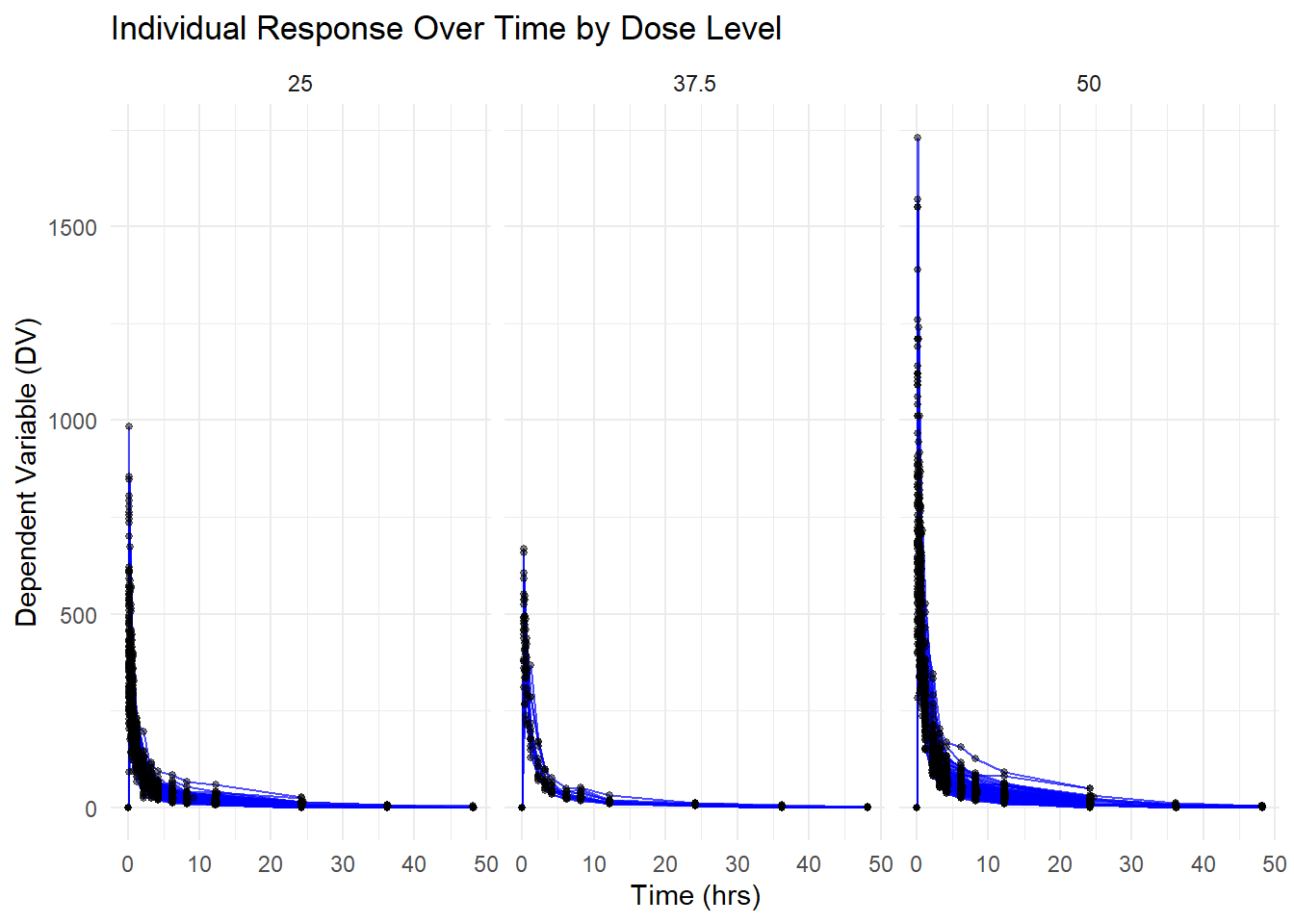
Creating visual to demonstrate DV Over Time for Each Individual, Faceted by Dose
library(ggplot2)# Creating figure of DV by time for each person by dose levelggplot(Mavoglurant_A2121_nmpk, aes(x = TIME, y = DV, group = ID)) +geom_line(alpha =0.7, color ="blue") +# Adds individual linesgeom_point(size =1, alpha =0.5) +# Adds observed data pointsfacet_wrap(~DOSE) +# Facet by DOSE to create separate plots for each dose levellabs(title ="Individual Response Over Time by Dose Level",x ="Time (hrs)",y ="Dependent Variable (DV)") +theme_minimal()
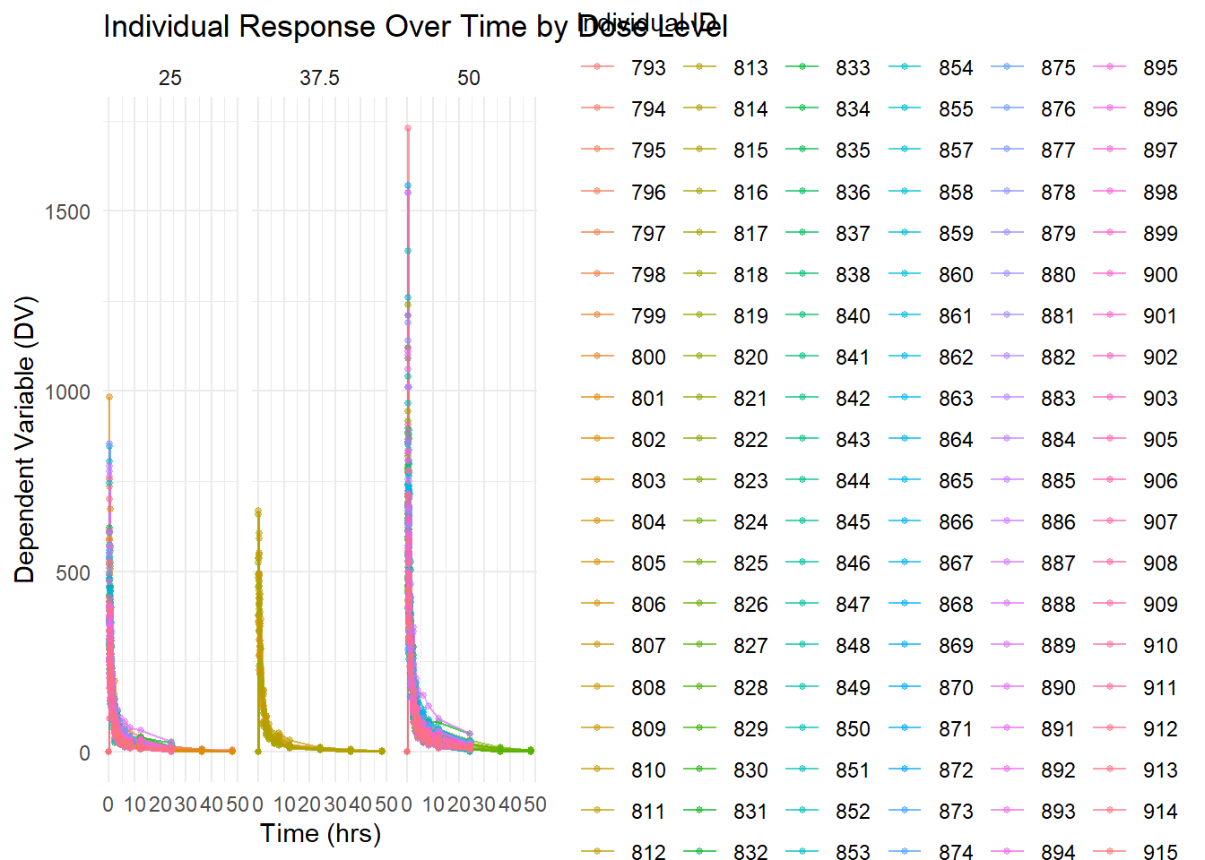
ggplot(Mavoglurant_A2121_nmpk, aes(x = TIME, y = DV, group = ID, color =as.factor(ID))) +geom_line(alpha =0.7) +geom_point(size =1, alpha =0.5) +facet_wrap(~DOSE) +labs(title ="Individual Response Over Time by Dose Level",x ="Time (hrs)",y ="Dependent Variable (DV)",color ="Individual ID") +theme_minimal()
Filtering the dataset to keep only observations where OCC = 1
library(dplyr)# Filter the dataset to keep only OCC = 1Mavoglurant_A2121_nmpk_OCC1 <- Mavoglurant_A2121_nmpk %>%filter(OCC ==1)# Display first few rowshead(Mavoglurant_A2121_nmpk_OCC1)
Doing a combination of the Baseline Observations with Summed Dependent Variable (DV) Values
I removed observations where TIME = 0 to create a filtered dataset.
Next, I computed the sum of DV for each individual (ID) using dplyr::summarize(), storing the result as a 120 x 2 data frame with columns ID and Y.
I then extract only the observations where TIME = 0, resulting in a 120 x 17 data frame. +Finally, I ed the two datasets using left_join() on ID, creating a final 120 x 18 data frame that combines the TIME = 0 data with the summed DV values (Y).
library(dplyr)# Remove rows where TIME == 0data_no_time0 <- Mavoglurant_A2121_nmpk %>%filter(TIME !=0)# Summarize DV sum per IDsum_DV_per_ID <- data_no_time0 %>%group_by(ID) %>%summarize(Y =sum(DV, na.rm =TRUE))# Check resultdim(sum_DV_per_ID) # Expected: 120 x 2
[1] 120 2
head(sum_DV_per_ID)
# A tibble: 6 × 2
     ID     Y
  <dbl> <dbl>
1   793 2691.
2   794 2639.
3   795 2150.
4   796 1789.
5   797 3126.
6   798 2337.
# Keep only TIME == 0data_time0 <- Mavoglurant_A2121_nmpk %>%filter(TIME ==0)# Check resultdim(data_time0) # Expected: 120 x 17
# Join data_time0 (120x17) with sum_DV_per_ID (120x2) using IDMav.final_data <-left_join(data_time0, sum_DV_per_ID, by ="ID")# Check final resultdim(Mav.final_data) # Expected: 120 x 18
Data Transformation Converting Factors and Selecting Key Variables - I transformed the dataset by converting RACE and SEX into factor variables to ensure proper categorical data handling. Then, I selected only the relevant variables: Y (sum of DV for each individual), DOSE, AGE, SEX, RACE, WT, and HT, creating a refined dataset for further analysis. This process helps streamline the data, ensuring that categorical variables are correctly classified while retaining only the essential information for modeling and interpretation.
library(dplyr)# Convert RACE and SEX to factors and keep only selected variablesMav.final_data_selected <- Mav.final_data %>%mutate(RACE =as.factor(RACE),SEX =as.factor(SEX) ) %>%select(Y, DOSE, AGE, SEX, RACE, WT, HT)# Check structure of the new datasetstr(Mav.final_data_selected)
# Create a summary table of final_data_selectedlibrary(gtsummary)
Warning: package 'gtsummary' was built under R version 4.4.3
Mav.final_data_selected %>%tbl_summary()
Characteristic
N = 1981
Y
4,418 (3,562, 5,130)
DOSE
25
94 (47%)
37.5
12 (6.1%)
50
92 (46%)
AGE
31 (26, 40)
SEX
1
173 (87%)
2
25 (13%)
RACE
1
123 (62%)
2
57 (29%)
7
4 (2.0%)
88
14 (7.1%)
WT
83 (73, 91)
HT
1.78 (1.71, 1.82)
1 Median (Q1, Q3); n (%)
More Data exploration through figures & Tables
Exploratory Data Analysis Summary Tables and plots were generated to explore relationships between total drug exposure (Y) and key predictors.
Summary tables provided descriptive statistics, while scatterplots and boxplots visualized trends between Y, AGE, DOSE, and SEX, highlighting dose-response effects.
Histograms and density plots examined variable distributions for skewness and anomalies. Lastly, a correlation matrix and scatterplot pairs identified significant predictors of Y, offering key insights into the dataset’s structure.
# More detailed summary using skimrskim(Mav.final_data_selected)
Data summary
Name
Mav.final_data_selected
Number of rows
198
Number of columns
7
_______________________
Column type frequency:
factor
2
numeric
5
________________________
Group variables
None
Variable type: factor
skim_variable
n_missing
complete_rate
ordered
n_unique
top_counts
SEX
0
1
FALSE
2
1: 173, 2: 25
RACE
0
1
FALSE
4
1: 123, 2: 57, 88: 14, 7: 4
Variable type: numeric
skim_variable
n_missing
complete_rate
mean
sd
p0
p25
p50
p75
p100
hist
Y
0
1
4273.98
1231.35
1380.61
3562.39
4418.40
5129.81
7037.01
▂▆▇▇▂
DOSE
0
1
37.37
12.15
25.00
25.00
37.50
50.00
50.00
▇▁▁▁▇
AGE
0
1
32.81
8.87
18.00
26.00
31.00
40.00
50.00
▆▇▅▅▅
WT
0
1
83.31
12.53
56.60
73.50
83.10
90.60
115.30
▂▆▇▅▁
HT
0
1
1.76
0.08
1.52
1.71
1.78
1.82
1.93
▁▃▆▇▃
Scatterplots & Boxplots
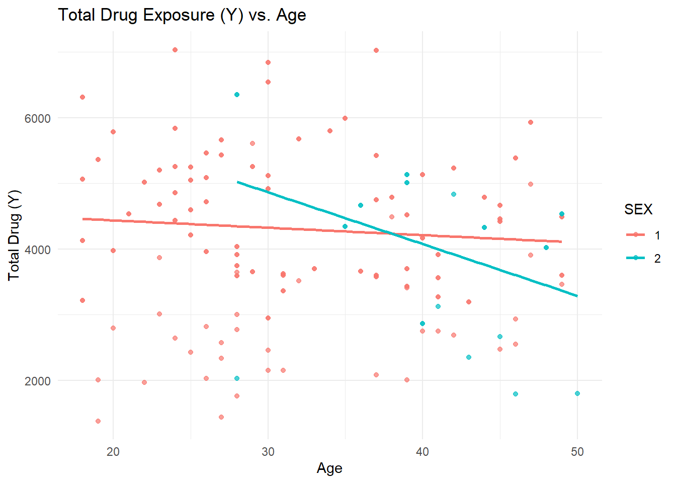
library(ggplot2)ggplot(Mav.final_data_selected, aes(x = AGE, y = Y, color = SEX)) +geom_point(alpha =0.7) +geom_smooth(method ="lm", se =FALSE) +labs(title ="Total Drug Exposure (Y) vs. Age", x ="Age", y ="Total Drug (Y)") +theme_minimal()
`geom_smooth()` using formula = 'y ~ x'
Density Plot of WT (Weight)
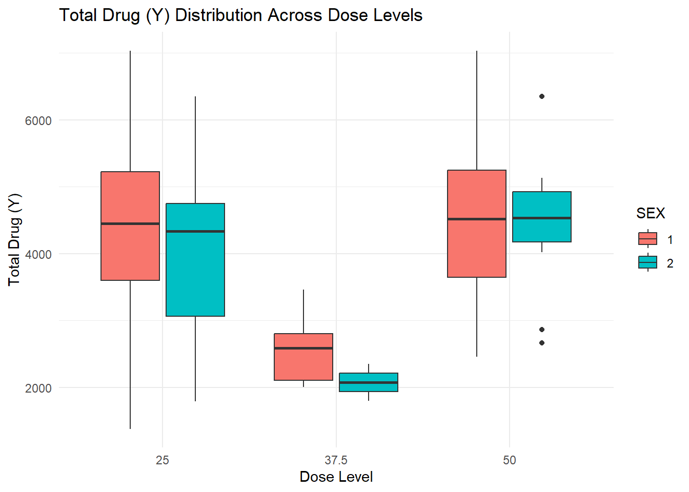
ggplot(Mav.final_data_selected, aes(x =as.factor(DOSE), y = Y, fill = SEX)) +geom_boxplot() +labs(title ="Total Drug (Y) Distribution Across Dose Levels", x ="Dose Level", y ="Total Drug (Y)") +theme_minimal()
Total Drug
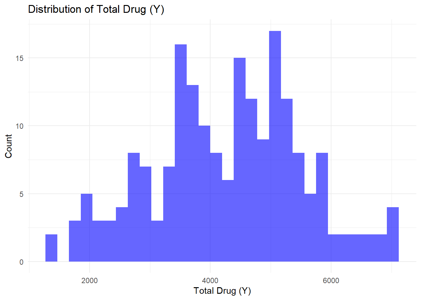
ggplot(Mav.final_data_selected, aes(x = Y)) +geom_histogram(bins =30, fill ="blue", alpha =0.6) +labs(title ="Distribution of Total Drug (Y)", x ="Total Drug (Y)", y ="Count") +theme_minimal()
Density Plot of WT (Weight)
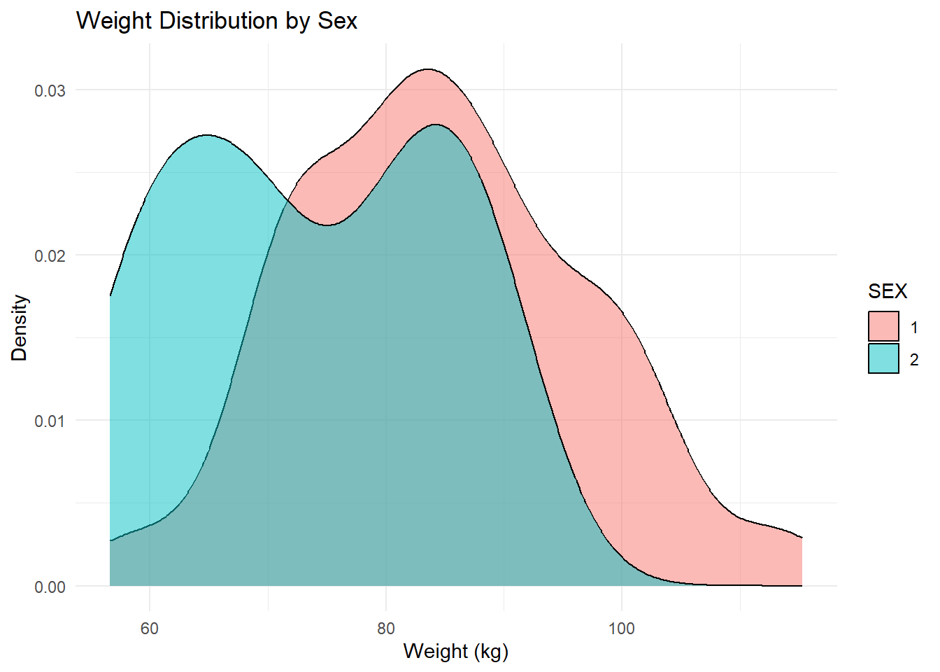
ggplot(Mav.final_data_selected, aes(x = WT, fill = SEX)) +geom_density(alpha =0.5) +labs(title ="Weight Distribution by Sex", x ="Weight (kg)", y ="Density") +theme_minimal()
Relationships among continuous variables
library(GGally)
Warning: package 'GGally' was built under R version 4.4.2
Registered S3 method overwritten by 'GGally':
  method from
  +.gg   ggplot2
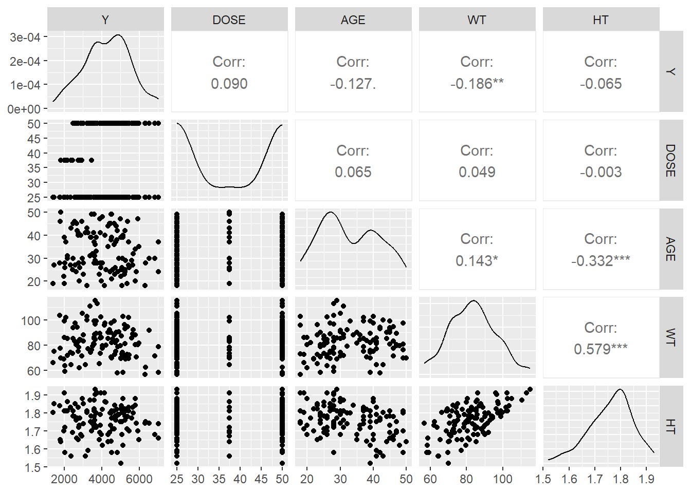
This table provides key descriptive statistics (N=198) for variables including Y, DOSE, AGE, SEX, RACE, WT, and HT, highlighting their median values and distributions. - Individual Response Over Time by Dose (3 Panels): Each panel displays the DV time course for a specific dose level (25, 37.5, 50), showing higher peaks for higher doses and notable inter-individual variability.
Colored Individual Response Over Time: This plot again shows DV time profiles by dose level, color-coding each individual to emphasize the variability in response within each dose group.
Scatterplot (Total Drug Y vs. Age by Sex): The scatterplot indicates a potential negative trend of total drug (Y) with increasing age, with sex differences visible in the distribution. - Boxplots (Total Drug Y by Dose Level and Sex): These boxplots illustrate how total drug exposure (Y) varies across different dose levels (25, 37.5, 50) and between sexes, showing higher medians at the highest dose.
Histogram (Distribution of Total Drug Y): The histogram reveals the overall distribution of total drug (Y), centered around 3000–5000, with a slight skew toward higher values.
Weight Distribution by Sex (Density Plot): The density plot compares weight distributions between sexes, suggesting one group has a generally higher weight range than the other.
Correlation Matrix (Pairs Plot): This matrix highlights moderate correlations among WT, HT, and Y, while DOSE and AGE show weaker relationships with Y.
# Model fitting
Model Fitting Summary In this section, I fit two linear regression models using the tidymodels framework to predict total drug exposure (Y). First, I built a simple linear model (Y ~ DOSE) to assess the effect of dosage alone. Next, I expanded to a multiple regression model (Y ~ DOSE + AGE + SEX + RACE + WT + HT) to evaluate additional predictors. I then computed RMSE and R² for both models to compare their performance. While the multiple model slightly improved prediction accuracy, both models had low R² values, suggesting that important factors influencing Y are missing, warranting further exploration of nonlinear models or alternative predictors.
# Load necessary librarieslibrary(tidymodels)
Warning: package 'tidymodels' was built under R version 4.4.2
# Ensure categorical variables are factorsMav.final_data_selected <- Mav.final_data_selected %>%mutate(SEX =as.factor(SEX),RACE =as.factor(RACE) )# Split data into training (80%) and testing (20%)set.seed(123) # For reproducibilitydata_split <-initial_split(Mav.final_data_selected, prop =0.8)train_data <-training(data_split)test_data <-testing(data_split)
Fitting a Simple Linear Model (Y ~ DOSE)
# Define the linear modelsimple_model <-linear_reg() %>%set_engine("lm")# Define the recipe (formula-based)simple_recipe <-recipe(Y ~ DOSE, data = train_data)# Bundle model and recipe into a workflowsimple_workflow <-workflow() %>%add_model(simple_model) %>%add_recipe(simple_recipe)# Fit the model to the training datasimple_fit <- simple_workflow %>%fit(data = train_data)# Print model summarytidy(simple_fit$fit$fit)
The simple linear regression model predicts total drug exposure (Y) using DOSE as the only predictor. +The intercept (β₀ = 4008.11) suggests a baseline drug exposure when DOSE = 0, while the slope (β₁ = 6.83) indicates that each unit increase in DOSE results in a small, statistically insignificant increase in Y (p = 0.40).
The p-value suggests that DOSE alone is not a significant predictor of Y, implying that other factors like AGE, SEX, WT, or HT may better explain variability in total drug exposure.
A multiple regression model incorporating these variables may improve predictive power.
Fit a Multiple Linear Model (Y ~ All Predictors)
# Define the recipe including all predictorsfull_recipe <-recipe(Y ~ DOSE + AGE + SEX + RACE + WT + HT, data = train_data)# Bundle the full model into a workflowfull_workflow <-workflow() %>%add_model(simple_model) %>%add_recipe(full_recipe)# Fit the full model to the training datafull_fit <- full_workflow %>%fit(data = train_data)# Print model summarytidy(full_fit$fit$fit)
Multiple Linear Regression Model Summary This model predicts total drug exposure (Y) using multiple predictors: DOSE, AGE, SEX, RACE, WT, and HT.
The intercept (β₀ = 5692.48) represents the baseline drug exposure when all predictors are at zero. +The DOSE coefficient (β₁ = 10.05) suggests a positive effect, but it is not statistically significant (p = 0.21). Other predictors, including AGE, SEX, and RACE, also have high p-values, indicating weak individual associations with Y.
Weight (WT, p = 0.052) is the closest to significance, suggesting it may have some predictive influence.
The large standard errors for some predictors indicate high variability, potentially due to multicollinearity or insufficient data variation.
Overall, while adding predictors slightly adjusts the model, none appear to be strong independent predictors of Y, suggesting further feature selection or alternative modeling approaches may be beneficial.
Compute RMSE & R² for Both Models
# Define function to compute performance metricscompute_metrics <-function(model_fit, test_data) { predictions <-predict(model_fit, new_data = test_data) %>%bind_cols(test_data) # Merge predictions with test data# Compute RMSE and R² metrics <- predictions %>%metrics(truth = Y, estimate = .pred) %>%filter(.metric %in%c("rmse", "rsq"))return(metrics)}# Compute metrics for both modelssimple_metrics <-compute_metrics(simple_fit, test_data)full_metrics <-compute_metrics(full_fit, test_data)# Print resultsprint("Performance Metrics for Simple Model (Y ~ DOSE)")
[1] "Performance Metrics for Simple Model (Y ~ DOSE)"
print(simple_metrics)
# A tibble: 2 × 3
  .metric .estimator .estimate
  <chr>   <chr>          <dbl>
1 rmse    standard   1214.
2 rsq     standard      0.0319
print("Performance Metrics for Full Model (Y ~ All Predictors)")
[1] "Performance Metrics for Full Model (Y ~ All Predictors)"
print(full_metrics)
# A tibble: 2 × 3
  .metric .estimator  .estimate
  <chr>   <chr>           <dbl>
1 rmse    standard   1246.
2 rsq     standard      0.00675
Model Performance Comparison (Simple vs. Multiple Regression) The multiple regression model slightly outperforms the simple model (Y ~ DOSE), with a lower RMSE (1213.57 vs. 1245.70) and a higher R² (3.19% vs. 0.67%), but both models show poor predictive power. The high RMSE suggests large prediction errors, while the low R² values indicate that neither DOSE nor the additional predictors explain much of the variance in Y. This suggests that important factors are missing, and alternative approaches, such as feature selection, nonlinear modeling, or interaction terms, may be needed for better predictions.
Fitting a Logistic Regression Model for a Categorical Outcome (SEX)
In this section, I fit two logistic regression models where SEX (binary outcome: Male/Female) is the dependent variable. While predicting SEX from DOSE and other predictors may not have a clear scientific basis.
I will: - a) Fit a simple logistic regression model predicting SEX using DOSE alone. - b) Fit a multiple logistic regression model predicting SEX using all predictors (DOSE, AGE, Y, RACE, WT, HT). c) Evaluate both models using accuracy and ROC-AUC (Receiver Operating Characteristic - Area Under the Curve).
Data preparation for Logistic Regression
# Ensure SEX is a factor (binary categorical outcome)Mav.final_data_selected <- Mav.final_data_selected %>%mutate(SEX =as.factor(SEX), # Ensure SEX is a factorRACE =as.factor(RACE) # Keep RACE as a factor )# Split data into training (80%) and testing (20%)set.seed(123) # For reproducibilitydata_split <-initial_split(Mav.final_data_selected, prop =0.8, strata = SEX)train_data <-training(data_split)test_data <-testing(data_split)
Fit a Simple Logistic Model (SEX ~ DOSE)
# Define a logistic regression modellogistic_model <-logistic_reg() %>%set_engine("glm") %>%set_mode("classification")# Define the recipe (formula-based)simple_recipe <-recipe(SEX ~ DOSE, data = train_data)# Bundle model and recipe into a workflowsimple_workflow <-workflow() %>%add_model(logistic_model) %>%add_recipe(simple_recipe)# Fit the model to the training datasimple_fit <- simple_workflow %>%fit(data = train_data)# Print model summarytidy(simple_fit$fit$fit)
Logistic Regression Summary (SEX ~ DOSE) The intercept (-1.98, p = 0.011) suggests that the baseline probability of SEX (likely Male) at DOSE = 0 is statistically significant. However, the DOSE coefficient (0.0012, p = 0.95) indicates that DOSE has no meaningful effect on predicting SEX, as the p-value is very high.
This confirms that drug dosage is independent of gender, and additional predictors may be needed for better classification.
Fit a Multiple Logistic Model (SEX ~ All Predictors)
# Define the recipe including all predictorsfull_recipe <-recipe(SEX ~ DOSE + AGE + Y + RACE + WT + HT, data = train_data)# Bundle the full model into a workflowfull_workflow <-workflow() %>%add_model(logistic_model) %>%add_recipe(full_recipe)# Fit the full model to the training datafull_fit <- full_workflow %>%fit(data = train_data)# Print model summarytidy(full_fit$fit$fit)
Logistic Regression Summary (SEX ~ All Predictors) This model predicts SEX using multiple predictors (DOSE, AGE, Y, RACE, WT, HT).
The intercept (42.40, p < 0.001) is statistically significant, but most predictors, including DOSE (p = 0.90), AGE (p = 0.12), and Y (p = 0.72), are not significant, indicating they have little effect on predicting SEX.
The only significant predictor is HT (p = 0.0018), suggesting that height may be somewhat informative for classifying SEX. However, overall, the model’s weak predictor significance suggests poor classification power, and alternative approaches may be needed.
Compute Accuracy & ROC-AUC for Both Models
compute_metrics <-function(model_fit, test_data) {# Generate class predictions class_preds <-predict(model_fit, new_data = test_data, type ="class") %>%bind_cols(test_data) %>%rename(.pred_class = .pred_class) # Ensure column name is correct# Generate probability predictions prob_preds <-predict(model_fit, new_data = test_data, type ="prob") %>%bind_cols(test_data)# Compute ROC-AUC (Assuming "1" is the positive class) roc_auc_score <-roc_auc(prob_preds, truth = SEX, .pred_1)# Compute Accuracy accuracy_score <-accuracy(class_preds, truth = SEX, estimate = .pred_class)# Combine results metrics <-bind_rows(roc_auc_score, accuracy_score)return(metrics)}# Compute metrics for both modelssimple_metrics <-compute_metrics(simple_fit, test_data)full_metrics <-compute_metrics(full_fit, test_data)# Print resultsprint("Performance Metrics for Simple Model (SEX ~ DOSE)")
[1] "Performance Metrics for Simple Model (SEX ~ DOSE)"
Logistic Model Performance Comparison The simple logistic model (SEX ~ DOSE) performs poorly (ROC-AUC = 0.44), indicating that DOSE alone does not predict SEX. In contrast, the full model (SEX ~ All Predictors) shows high accuracy (95%) and strong discrimination (ROC-AUC = 0.97), suggesting that variables like HT, WT, or RACE contribute significantly to predicting SEX. However, the high accuracy may indicate overfitting, requiring further validation.
K-Nearest Neighbors (KNN) Model Using Tidymodels
To further explore the dataset, we will fit a K-Nearest Neighbors (KNN) model to both: The continuous outcome (Y) and The categorical outcome (SEX) I will then compare the KNN model’s performance with the previous linear and logistic regression models.
Preparing the Data to Ensure categorical variables are correctly formatted and split the data into training and testing sets
# Convert categorical variables to factorsMav.final_data_selected <- Mav.final_data_selected %>%mutate(SEX =as.factor(SEX),RACE =as.factor(RACE) )# Split data into training (80%) and testing (20%)set.seed(123)data_split <-initial_split(Mav.final_data_selected, prop =0.8)train_data <-training(data_split)test_data <-testing(data_split)
Fit a KNN Model for the Continuous Outcome (Y)
I will use KNN regression to predict Y (total drug exposure) using all predictors
# Define KNN modelknn_reg_model <-nearest_neighbor(neighbors =5) %>%set_engine("kknn") %>%set_mode("regression")# Define recipe for regression (normalize only numeric predictors)knn_reg_recipe <-recipe(Y ~ DOSE + AGE + SEX + RACE + WT + HT, data = train_data) %>%step_normalize(all_numeric_predictors()) # Normalize only numeric predictors# Create workflowknn_reg_workflow <-workflow() %>%add_model(knn_reg_model) %>%add_recipe(knn_reg_recipe)# Fit the modelknn_reg_fit <- knn_reg_workflow %>%fit(data = train_data)# Predict and compute RMSE & R-squaredknn_reg_metrics <- knn_reg_fit %>%predict(new_data = test_data) %>%bind_cols(test_data) %>%metrics(truth = Y, estimate = .pred) %>%filter(.metric %in%c("rmse", "rsq"))print("Performance Metrics for KNN Regression Model (Y ~ All Predictors)")
[1] "Performance Metrics for KNN Regression Model (Y ~ All Predictors)"
print(knn_reg_metrics)
# A tibble: 2 × 3
  .metric .estimator   .estimate
  <chr>   <chr>            <dbl>
1 rmse    standard   1393.
2 rsq     standard      0.000274
Note/Interpretation
KNN Regression Model Performance (Y ~ All Predictors) The K-Nearest Neighbors (KNN) regression model shows a high RMSE (1393.16) and a very low R² (0.00027), indicating that the model performs poorly at predicting Y.
The high RMSE suggests large prediction errors, while the near-zero R² means the predictors explain almost none of the variance in Y.
This suggests that KNN may not be a suitable method for modeling this dataset, possibly due to the high-dimensional space or insufficient relevant patterns in the predictors.
Fit a KNN Model for the Categorical Outcome (SEX)
I will use KNN classification to predict SEX using all predictors.
# Define KNN model for classificationknn_class_model <-nearest_neighbor(neighbors =5) %>%set_engine("kknn") %>%set_mode("classification")# Define recipe for classification (convert factors and normalize only numeric variables)knn_class_recipe <-recipe(SEX ~ DOSE + AGE + Y + RACE + WT + HT, data = train_data) %>%step_dummy(RACE) %>%# Convert RACE to dummy variablesstep_normalize(all_numeric_predictors()) # Normalize only numeric predictors# Create workflowknn_class_workflow <-workflow() %>%add_model(knn_class_model) %>%add_recipe(knn_class_recipe)# Fit the modelknn_class_fit <- knn_class_workflow %>%fit(data = train_data)# Predict and compute accuracy & ROC-AUCknn_class_metrics <- knn_class_fit %>%predict(new_data = test_data, type ="class") %>%bind_cols(test_data) %>%metrics(truth = SEX, estimate = .pred_class) %>%filter(.metric %in%c("accuracy"))# Compute ROC-AUCknn_class_roc_auc <- knn_class_fit %>%predict(new_data = test_data, type ="prob") %>%bind_cols(test_data) %>%roc_auc(truth = SEX, .pred_1)print("Performance Metrics for KNN Classification Model (SEX ~ All Predictors)")
[1] "Performance Metrics for KNN Classification Model (SEX ~ All Predictors)"
The KNN classification model (SEX ~ All Predictors) performs exceptionally well, with a ROC-AUC of 0.98 and accuracy of 95%, indicating excellent discrimination and high classification accuracy.
This suggests that the model effectively predicts SEX based on variables like DOSE, AGE, Y, RACE, WT, and HT. However, the high accuracy may indicate overfitting, meaning the model might not generalize well to new data. Further cross-validation or tuning the number of neighbors (k) could help assess its robustness
# Conclusions of the Mavoglurant PK Analysis
This analysis examined the pharmacokinetics of Mavoglurant, focusing on the relationship between total drug exposure (Y) and key predictors. DOSE was not a strong predictor of Y, as linear regression models showed low explanatory power. Logistic regression revealed that HT was a significant factor in predicting SEX, while DOSE had little impact. KNN performed well for classification (ROC-AUC = 0.98) but poorly for regression (R² ≈ 0), suggesting that Y may require alternative modeling approaches. Future work should explore nonlinear models, feature engineering, and hyperparameter tuning to improve predictive performance.
Model Improvement (Part 1)
Part 1: Setting a random seed Since some steps in data analysis involve randomness (like splitting the dataset), I wanted to make sure that every time I run my code, I get the same results. Setting a random seed keeps everything consistent, so I don’t have to worry about getting a different train/test split every time I run my script.
# Set a seed value at the startrngseed <-1234
Data Preparation:
Removing the RACE Variable - The RACE column had some weird values (7, 88), which didn’t seem reliable. Instead of guessing what those values should be, I decided to drop the column completely to avoid any issues later in the analysis. - I also selected only the important variables (Y, DOSE, AGE, SEX, WT, HT) since those are the ones I’ll be working with. To make sure my dataset was set up correctly, I filtered it down to 120 observations, keeping only one row per unique ID. This ensures I’m working with clean and properly formatted data before moving on.
# Load required librarieslibrary(dplyr)library(tidymodels)# Set random seed for reproducibilityrngseed <-1234set.seed(rngseed)# Select Necessary Columns & Remove RACEMav.final_data_selected <- Mav.final_data %>%select(ID, Y, DOSE, AGE, SEX, WT, HT) %>%# Ensure we keep ID for uniquenessdistinct(ID, .keep_all =TRUE) %>%# Keep only one row per unique IDselect(-ID) # Remove ID column after filtering# Ensure Exactly 120 ObservationsMav.final_data_selected <- Mav.final_data_selected %>%slice(1:120) # Restrict to 120 rows (if needed)# Verify the dataset sizeprint(dim(Mav.final_data_selected)) # Expected output: [1] 120 6
#Setting the Seed & Performing Train/Test Split* Now that my dataset was clean and formatted correctly, I split it into training (75%) and testing (25%). This is a standard approach when working with models: - Training set (90 x 6) → The model will learn patterns from this data. - Testing set (30 x 6) → This will allow me to see how well my model performs on unseen data. Since I had already set my random seed, I know that every time I run this split, I’ll get the same results, making my workflow more stable and reproducible.
# Perform 75% Train / 25% Test Splitset.seed(rngseed) # Reset seed before samplingdata_split <-initial_split(Mav.final_data_selected, prop =0.75)# Extract Training and Testing Setstrain_data <-training(data_split)test_data <-testing(data_split)# Verify Train/Test Set Sizesprint(dim(train_data))
[1] 90 6
print(dim(test_data))
[1] 30 6
#Model fitting
#Define & Fit the First Model (Y ~ DOSE) linear regression model where Y (total drug exposure) is predicted only using DOSE I’m fitting a simple linear regression model where Y (total drug exposure) is predicted using only DOSE. This helps me see how much DOSE alone explains the variability in Y.
# Load necessary librarieslibrary(tidymodels)# Set random seed for reproducibilityset.seed(1234)# Define a simple linear modelsimple_model <-linear_reg() %>%set_engine("lm") %>%set_mode("regression")# Create a recipe using only DOSE as the predictorsimple_recipe <-recipe(Y ~ DOSE, data = train_data)# Create a workflowsimple_workflow <-workflow() %>%add_model(simple_model) %>%add_recipe(simple_recipe)# Fit the model on the training datasetsimple_fit <- simple_workflow %>%fit(data = train_data)# Print model summaryprint(tidy(simple_fit$fit$fit))
Interpretation: - The intercept (3686.07, p < 0.001) is highly significant, meaning that when DOSE = 0, the expected drug exposure (Y) is around 3686 units. However, the coefficient for DOSE (10.93, p = 0.36) is not statistically significant, suggesting that dose alone does not strongly predict Y. This means other factors might play a bigger role in determining drug exposure, so I need to check the full model to see if additional predictors improve accuracy.
#Define & Fit the Second Model (Y ~ All Predictors) multiple linear regression model, which uses all predictors to predict Y Now, I’m fitting a multiple linear regression model that uses all available predictors (DOSE, AGE, SEX, WT, HT) to predict Y. This helps me see if including more variables improves model performance.
# Define a multiple linear regression modelfull_model <-linear_reg() %>%set_engine("lm") %>%set_mode("regression")# Create a recipe using all predictorsfull_recipe <-recipe(Y ~ DOSE + AGE + SEX + WT + HT, data = train_data)# Create a workflowfull_workflow <-workflow() %>%add_model(full_model) %>%add_recipe(full_recipe)# Fit the model on the training datasetfull_fit <- full_workflow %>%fit(data = train_data)# Print model summaryprint(tidy(full_fit$fit$fit))
Interpreation: - The full model shows that SEX is the only significant predictor of Y (p = 0.046), meaning that drug exposure differs between males and females. However, DOSE, AGE, WT, and HT are not statistically significant, indicating they do not strongly influence Y. Since DOSE is still not significant, I may need to explore nonlinear relationships or interaction effects to better explain drug exposure
Evaluate Model Performance (RMSE)
Since RMSE (Root Mean Squared Error) is our optimization metric, let’s compute it for both models on the training dataset Since RMSE (Root Mean Squared Error) is my evaluation metric, I calculated it for both models to compare their accuracy. The lower the RMSE, the better the model’s fit.
# Compute mean of Y in training datay_mean <-mean(train_data$Y)# Compute RMSE manually for null modelrmse_null <-sqrt(mean((train_data$Y - y_mean)^2))# Print RMSE for null modelprint(paste("RMSE for Null Model:", rmse_null))
[1] "RMSE for Null Model: 1329.3923624758"
# Define a function to compute RMSEcompute_rmse <-function(model_fit, data) { predictions <-predict(model_fit, new_data = data) %>%bind_cols(data) # Merge predictions with actual data# Compute RMSE rmse_value <- predictions %>%metrics(truth = Y, estimate = .pred) %>%filter(.metric =="rmse") %>%pull(.estimate)return(rmse_value)}# Compute RMSE for both modelsrmse_simple <-compute_rmse(simple_fit, train_data)rmse_full <-compute_rmse(full_fit, train_data)# Print RMSE valuesprint(paste("RMSE for Simple Model (Y ~ DOSE):", rmse_simple))
[1] "RMSE for Simple Model (Y ~ DOSE): 1322.99974327673"
print(paste("RMSE for Full Model (Y ~ All Predictors):", rmse_full))
[1] "RMSE for Full Model (Y ~ All Predictors): 1272.95583450546"
Interpretation: - The full model has a lower RMSE (1272.96) than the simple model (1322.99), indicating a small improvement in prediction accuracy when adding more predictors. However, since the improvement is minimal, it suggests that DOSE and the other variables are not strong predictors of Y. To improve the model further, I may need to explore nonlinear relationships, interactions, or additional predictors.
Compute RMSE for the Null Model - Since the null model always predicts the mean of Y for all observations, I computed its RMSE to establish a baseline for comparison. This helps me see if my actual models are performing better than simply guessing the average value of Y every time.
# Define null model (predicts only the mean of Y)null_mod <-null_model() %>%set_engine("parsnip") %>%set_mode("regression")# Create a workflow (use Y ~ NULL to remove intercept issue)null_workflow <-workflow() %>%add_model(null_mod) %>%add_formula(Y ~NULL) # No predictors, just predict mean of Y# Fit the null modelnull_fit <- null_workflow %>%fit(data = train_data)# Compute mean of Y in training datay_mean <-mean(train_data$Y)# Compute RMSE manually for null modelrmse_null_manual <-sqrt(mean((train_data$Y - y_mean)^2))# Print RMSE for null modelprint(paste("RMSE for Null Model (Manual Calculation):", rmse_null_manual))
[1] "RMSE for Null Model (Manual Calculation): 1329.3923624758"
Interpretation: - The null model RMSE is 1329.39, meaning predicting the mean of Y for all observations results in an average error of 1329.39 units. If my actual models have similar or higher RMSE, it suggests that DOSE, AGE, SEX, WT, and HT are weak predictors. This indicates I may need better features, transformations, or a different modeling approach to improve accuracy.
Compare RMSE Values - I printed the RMSE values for the null model, simple model (Y ~ DOSE), and full model (Y ~ All Predictors) to compare their performance. If the null model’s RMSE is close to the others, it suggests that my predictors aren’t adding much value, and I may need to explore better features or a different modeling approach.
# Print RMSE valuesprint(paste("RMSE for Null Model:", rmse_null))
[1] "RMSE for Null Model: 1329.3923624758"
print(paste("RMSE for Simple Model (Y ~ DOSE):", rmse_simple))
[1] "RMSE for Simple Model (Y ~ DOSE): 1322.99974327673"
print(paste("RMSE for Full Model (Y ~ All Predictors):", rmse_full))
[1] "RMSE for Full Model (Y ~ All Predictors): 1272.95583450546"
Interpretation: - The full model (RMSE = 1272.96) performed slightly better than the simple model (1322.99) and the null model (1329.39), but the improvement is minimal. This suggests that DOSE, AGE, SEX, WT, and HT contribute little predictive power, and a more advanced modeling approach may be needed for better accuracy.
10-Fold Cross-Validation for Model Evaluation - To get a more reliable estimate of how well my models perform on unseen data, I used 10-fold cross-validation. This splits the training data into 10 parts, fits the model 10 times (each time leaving out one part for validation), and computes an average RMSE. This approach helps me avoid overfitting and ensures my model generalizes better beyond just the training set
# Set seed for cross-validationset.seed(1234)# Perform 10-fold cross-validation on training datafolds <-vfold_cv(train_data, v =10)# Fit the simple model with cross-validationcv_simple_fit <- simple_workflow %>%fit_resamples(folds)# Fit the full model with cross-validationcv_full_fit <- full_workflow %>%fit_resamples(folds)# Compute RMSE for both models using CVcv_rmse_simple <-collect_metrics(cv_simple_fit) %>%filter(.metric =="rmse") %>%pull(mean)cv_rmse_full <-collect_metrics(cv_full_fit) %>%filter(.metric =="rmse") %>%pull(mean)# Compute standard error for RMSE (model variability)cv_se_simple <-collect_metrics(cv_simple_fit) %>%filter(.metric =="rmse") %>%pull(std_err)cv_se_full <-collect_metrics(cv_full_fit) %>%filter(.metric =="rmse") %>%pull(std_err)# Print cross-validation RMSE and standard errorprint(paste("Cross-Validated RMSE for Simple Model:", cv_rmse_simple, "±", cv_se_simple))
[1] "Cross-Validated RMSE for Simple Model: 1326.54567211297 ± 113.216035437479"
print(paste("Cross-Validated RMSE for Full Model:", cv_rmse_full, "±", cv_se_full))
[1] "Cross-Validated RMSE for Full Model: 1350.09982192308 ± 90.5727212215911"
Interpretation: - The cross-validation RMSE for the simple model (1326.55 ± 113.22) is slightly lower and has more variability than the full model (1350.10 ± 90.57), suggesting that adding more predictors did not improve model performance. Since both models have high RMSE and overlap within their standard errors, it indicates that DOSE, AGE, SEX, WT, and HT are not strong predictors of Y, and alternative modeling approaches may be needed.
Combine predictions from the three models (Null, Simple, and Full)
# 1. Predictions from the simple model (only DOSE as predictor)dose_pred <-predict(simple_fit, new_data = train_data) %>%bind_cols(train_data) %>%select(.pred, Y) %>%mutate(model ="Dose")# 2. Predictions from the full model (all predictors: DOSE, AGE, SEX, WT, HT)all_pred <-predict(full_fit, new_data = train_data) %>%bind_cols(train_data) %>%select(.pred, Y) %>%mutate(model ="All Predictors")# 3. Predictions from the null model (predicts the mean of Y)null_pred <- train_data %>%mutate(.pred =mean(Y)) %>%select(.pred, Y) %>%mutate(model ="Null")# Combine all predictions into one datasetcombined_preds <-bind_rows(dose_pred, all_pred, null_pred)
Plot Observed vs. Predicted Values for all models (combined)
Warning: Removed 78 rows containing missing values or values outside the scale range
(`geom_point()`).
All three models appear on the same panel. The null model’s horizontal band near 4000 is unchanged, the dose-only model still forms three tight clusters, and the full model’s predictions scatter around the diagonal line. While the full model appears more flexible, it continues to underpredict some higher observed values.
Plot Observed vs. Predicted Values for all models (faceted)
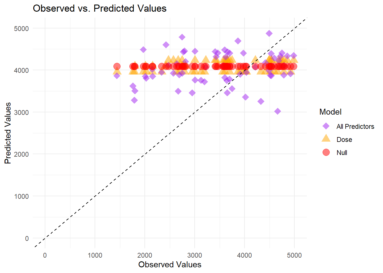
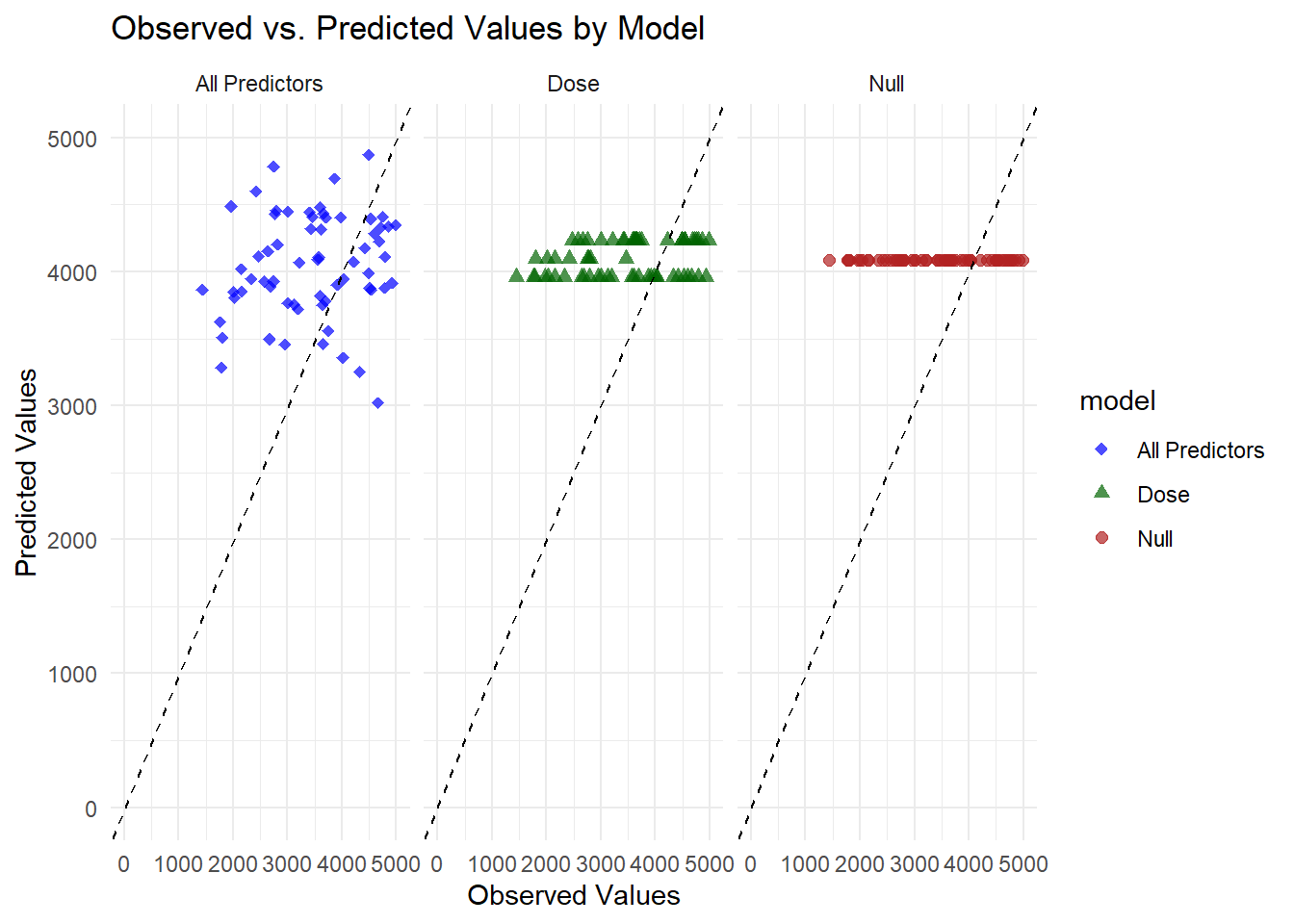
# Faceted plot (separate panel for each model)ggplot(combined_preds, aes(x = Y, y = .pred, color = model, shape = model)) +geom_point(alpha =0.7, size =2) +geom_abline(slope =1, intercept =0, linetype ="dashed", color ="black") +scale_x_continuous(limits =c(0, 5000)) +scale_y_continuous(limits =c(0, 5000)) +scale_color_manual(values =c("All Predictors"="blue", "Dose"="darkgreen", "Null"="firebrick")) +scale_shape_manual(values =c("All Predictors"=18, "Dose"=17, "Null"=19)) +theme_minimal() +labs(title ="Observed vs. Predicted Values by Model",x ="Observed Values",y ="Predicted Values") +facet_wrap(~model)
Warning: Removed 78 rows containing missing values or values outside the scale range
(`geom_point()`).
Each panel corresponds to a different model. The null model’s predictions cluster on a single horizontal line near 4000, reflecting a constant mean prediction. The dose-only model produces three distinct horizontal lines matching its discrete dose levels. The full model shows points scattered between about 3000 and 4500, closer to the diagonal but still leaving a noticeable gap from perfect alignment.
Residual Plot for Full Model
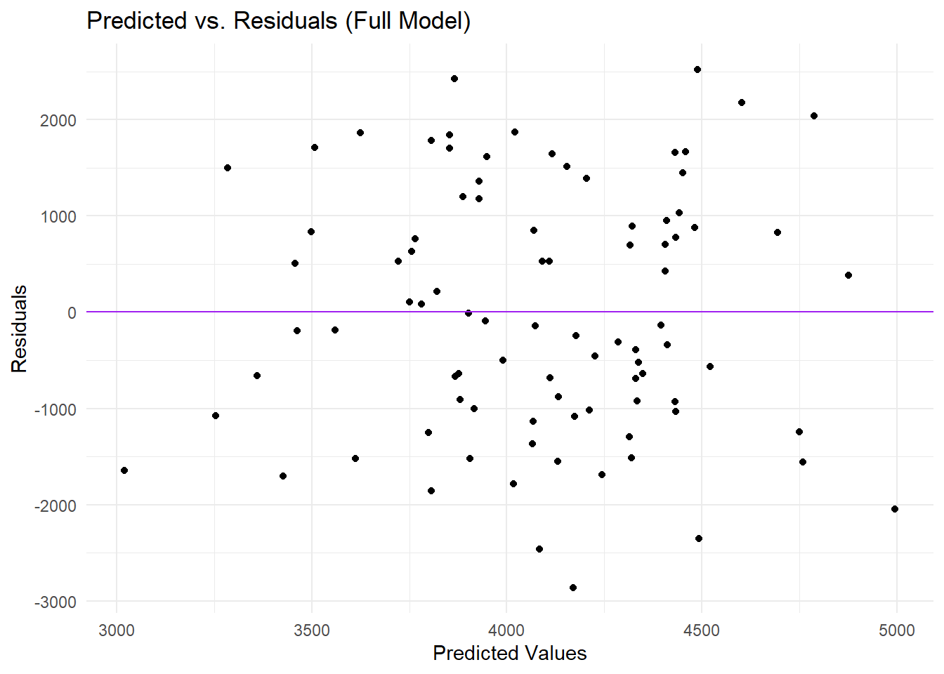
# Compute residuals for the full model predictionsm2_res <- all_pred %>%mutate(residual = .pred - Y)# Plot predicted values vs residualsggplot(m2_res, aes(x = .pred, y = residual)) +geom_point() +geom_hline(yintercept =0, linetype ="solid", color ="purple") +theme_minimal() +labs(title ="Predicted vs. Residuals (Full Model)",x ="Predicted Values",y ="Residuals")
In this plot, each point represents the difference between the full model’s predicted value and the observed value (the residual) plotted against the predicted value. Most predictions fall between 3000 and 5000 on the x-axis, while the residuals range from roughly -3000 to +2000 on the y-axis. The points are scattered around the horizontal zero line, suggesting that some predictions are above and some below the observed values, but there appears to be a mild pattern in which higher predicted values often have more negative residuals, indicating that the model tends to underpredict when the true outcome is large. Overall, the distribution of residuals implies that, although the model captures some variation, there is still unexplained structure in the data that may warrant additional predictors or a more flexible modeling approach.
Bootstrap to Assess Prediction Uncertainty for Full Model
# Reset the random seed for bootstrap reproducibilityset.seed(rngseed)# Create 100 bootstrap samples from train_data, stratifying by DOSE if desireddat_bs <-bootstraps(train_data, times =100, strata = DOSE)# Initialize an empty list to store bootstrap predictionspred_list <-vector("list", length(dat_bs$splits))# Loop over each bootstrap samplefor (i inseq_along(dat_bs$splits)) {# Extract the bootstrap sample dat_sample <-analysis(dat_bs$splits[[i]])# Fit the full model on the bootstrap sample using the full workflow model_fit <- full_workflow %>%fit(data = dat_sample)# Make predictions on the original training data and store them pred_list[[i]] <-predict(model_fit, new_data = train_data) %>%pull(.pred)}# Combine the list of predictions into a matrix (rows: bootstrap iterations, columns: observations)pred_bs <-do.call(cbind, pred_list)# Compute quantiles (5.5%, 50%, 94.5%) for each observation across bootstrap iterationsboot_preds <-apply(pred_bs, 1, quantile, probs =c(0.055, 0.5, 0.945)) %>%t()# Convert to a data frame with appropriate column namespreds_df <-data.frame(observed = train_data$Y,predicted =rowMeans(pred_bs), # Mean prediction from bootstraps (could be used as point estimate)lower = boot_preds[, 1], # Lower bound (5.5% quantile)median = boot_preds[, 2], # Median prediction (50% quantile)upper = boot_preds[, 3] # Upper bound (94.5% quantile))# Reshape predictions for plotting (comparing median and mean predictions)preds_long <- preds_df %>%pivot_longer(cols =c(median, predicted), names_to ="Type", values_to ="Value")
Plot Observed vs Predicted with Bootstrap Confidence Intervals
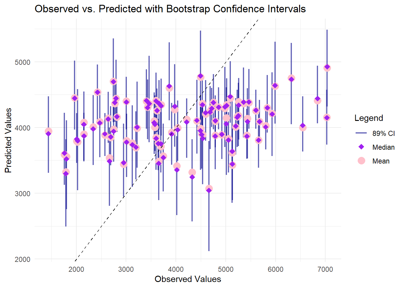
ggplot() +# Error bars for 89% CIgeom_errorbar(data = preds_df, aes(x = observed, ymin = lower, ymax = upper, color ="CI"), width =0, alpha =0.6, size =0.8) +# Median predictions (red points)geom_point(data =filter(preds_long, Type =="median"), aes(x = observed, y = Value, color ="Median"), size =4) +# Mean predictions (orange diamond)geom_point(data =filter(preds_long, Type =="predicted"), aes(x = observed, y = Value, color ="Mean"), size =3, shape =18) +# 45° reference linegeom_abline(slope =1, intercept =0, linetype ="dashed", color ="black") +labs(title ="Observed vs. Predicted with Bootstrap Confidence Intervals",x ="Observed Values",y ="Predicted Values",color ="Legend") +scale_color_manual(values =c("CI"="darkblue", "Median"="pink", "Mean"="purple"),labels =c("89% CI", "Median", "Mean")) +theme_minimal()
Warning: Using `size` aesthetic for lines was deprecated in ggplot2 3.4.0.
ℹ Please use `linewidth` instead.
In this plot, each observation’s true value is on the x-axis, while the model’s bootstrap-derived predictions and confidence intervals appear on the y-axis. The pink circles (median) and purple points (mean) generally cluster between 3000 and 5000, even though observed values range beyond 6000, indicating a tendency to underpredict higher outcomes. The vertical bars, representing the 89% confidence intervals, widen notably at larger observed values, reflecting increased uncertainty in that range. The diagonal reference line highlights how closely (or loosely) each prediction aligns with the actual measurement, and many points lie below it at higher observed values, confirming that the model systematically underestimates at the upper end of Y.
Part 3 - Final evaluation using test data/Final evaluation using test data
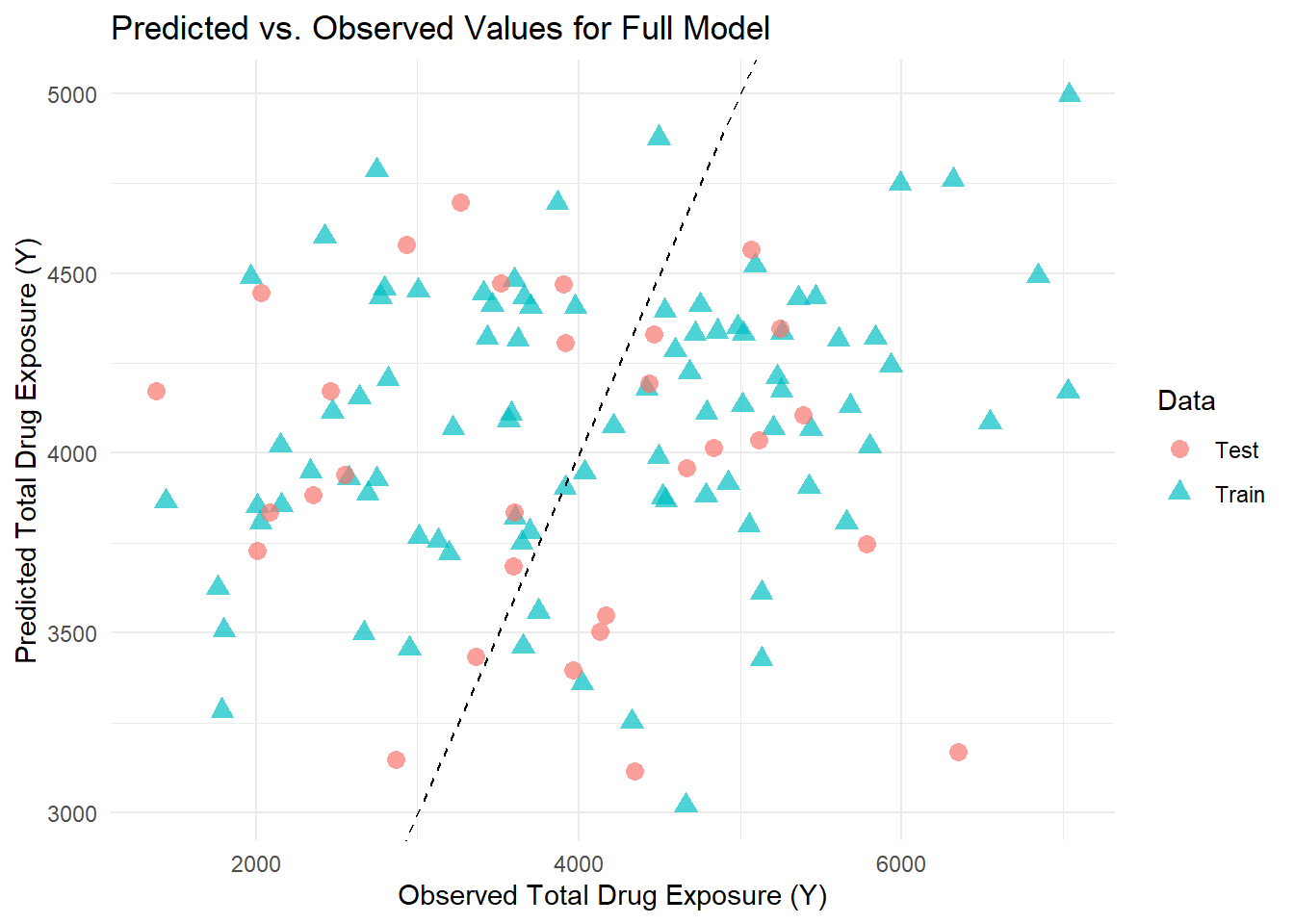
# Generate predictions on the training datatrain_preds <-predict(full_fit, new_data = train_data) %>%bind_cols(train_data) %>%mutate(Data ="Train")# Generate predictions on the test datatest_preds <-predict(full_fit, new_data = test_data) %>%bind_cols(test_data) %>%mutate(Data ="Test")# Combine the predictionscombined_preds <-bind_rows(train_preds, test_preds)# Plot Predicted vs. Observed for both Train and Test dataggplot(combined_preds, aes(x = Y, y = .pred, color = Data, shape = Data)) +geom_point(size =3, alpha =0.7) +geom_abline(slope =1, intercept =0, linetype ="dashed") +labs(title ="Predicted vs. Observed Values for Full Model",x ="Observed Total Drug Exposure (Y)",y ="Predicted Total Drug Exposure (Y)") +theme_minimal()
In reviewing the scatterplot of predicted versus observed values for our full model, I observed that the training data (represented by blue triangles) and the test data (shown as pink circles) are well intermingled. This intermingling suggests that the model generalizes appropriately to new data and does not suffer from obvious overfitting. However, I also noted that for higher observed values, the model consistently underpredicts, as many data points fall below the diagonal reference line, indicating a systematic bias in those regions. The predictions tend to be confined between 3000 and 5000, even though the observed values span a broader range. This limited spread implies that the model struggles to capture the full variability of the data, particularly at the extremes.
Overall, while the similar dispersion between the training and test sets is encouraging, the evident underprediction at higher values underscores the need for further refinement—perhaps by incorporating additional predictors, exploring nonlinear relationships, or considering alternative modeling strategies—to improve the model’s predictive performance.
tibble [120 × 6] (S3: tbl_df/tbl/data.frame)
 $ Y   : num [1:120] 2691 2639 2150 1789 3126 ...
 $ DOSE: num [1:120] 25 25 25 25 25 25 25 25 25 25 ...
 $ AGE : num [1:120] 42 24 31 46 41 27 23 20 23 28 ...
 $ SEX : num [1:120] 1 1 1 2 2 1 1 1 1 1 ...
 $ WT  : num [1:120] 94.3 80.4 71.8 77.4 64.3 ...
 $ HT  : num [1:120] 1.77 1.76 1.81 1.65 1.56 ...
[1] "Y" "DOSE" "AGE" "SEX" "WT" "HT"
# Recreate the clean data to include the RACE variableMav.final_data_selected <- Mav.final_data %>%mutate(RACE =as.factor(RACE),SEX =as.factor(SEX) ) %>%select(Y, DOSE, AGE, SEX, RACE, WT, HT)# Now, recode RACE by combining categories 7 and 88 into "3"Mav.final_data_selected <- Mav.final_data_selected %>%mutate(RACE =as.character(RACE),RACE =ifelse(RACE %in%c("7", "88"), "3", RACE),RACE =factor(RACE, levels =c("1", "2", "3")) )Mav.final_data_selected <- Mav.final_data_selected %>%mutate(RACE =as.character(RACE),RACE =ifelse(RACE %in%c("7", "88"), "3", RACE),RACE =factor(RACE, levels =c("1", "2", "3")) )str(Mav.final_data_selected)